Advanced Research WRF (ARW) Technical Note - MMM - University ...

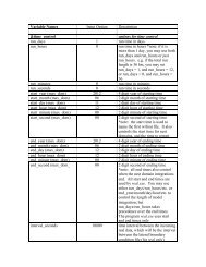
exception of the baroclinic wave test case, the sounding files are in text format that can be
directly edited by the user. The 1D specification of the sounding in these test files requires the
surface values of pressure, potential temperature, and water vapor mixing ratio, followed by the
potential temperature, vapor mixing ratio, and horizontal wind components at some heights
above the surface. The initialization programs for each case assume that this moist sounding
represents an atmosphere in hydrostatic balance.
Two sets of thermodynamic fields are needed for the model— the reference state and the
perturbation state (see Chapter 2 for further discussion of the equations). The reference state
used in the idealized initializations is computed using the input sounding from which the moisture
is discarded (because the reference state is dry). The perturbation state is computed using
the full moist input sounding. The procedure for computing the hydrostatically-balanced ARW
reference and perturbation state variables from the input sounding is as follows. First, density
and both a dry and full hydrostatic pressure are computed from the input sounding at the input
sounding levels z. This is accomplished by integrating the hydrostatic equation vertically up the
column using the surface pressure and potential temperature as the lower boundary condition.
The hydrostatic equation is
δzp = −ρ z g(1 + (Rd/Rv)q v z ), (5.1)
where ρ z is a two point average between input sounding levels, and δzp is the difference of
the pressure between input sounding levels divided by the height difference. Additionally, the
equation of state is needed to close the system:
αd = 1
ρd
= Rdθ
po
1 + Rd
qv
Rv
p
po
− cv
cp
, (5.2)
where qv and θ are given in the input sounding. (5.1) and (5.2) are a coupled set of nonlinear
equations for p and ρ in the vertical integration, and they are solved by iteration. The dry
pressure on input sounding levels is computed by integrating the hydrostatic relation down from
the top, excluding the vapor component.
Having computed the full pressure (dry plus vapor) and dry air pressure on the input sounding
levels, the pressure at the model top (pdht) is computed by linear interpolation in height
(or possibly extrapolation) given the height of the model top (an input variable). The column
mass µd is computed by interpolating the dry air pressure to the surface and subtracting it from
pdht. Given the column mass, the dry-air pressure at each η level is known from the coordinate
definition (2.1), repeated here
η = (pdh − pdht)/µd where µd = pdhs − pdht,
and the pressures pdhs and pdht refer to the dry atmosphere. The potential temperature from
the input sounding is interpolated to each of the model pressure levels, and the equation of state
(5.2) is used to compute the inverse density αd. Finally, the ARW’s hydrostatic relation (2.9),
in discrete form
δηφ = −αdµd
is used to compute the geopotential. This procedure is used to compute the reference state
(assuming a dry atmosphere) and the full state (using the full moist sounding). The perturbation
variables are computed as the difference between the reference and full state. It should also be
34