Advanced Research WRF (ARW) Technical Note - MMM - University ...
Advanced Research WRF (ARW) Technical Note - MMM - University ...
Advanced Research WRF (ARW) Technical Note - MMM - University ...

You also want an ePaper? Increase the reach of your titles
YUMPU automatically turns print PDFs into web optimized ePapers that Google loves.
of its useful life. The development of a unified global/regional <strong>WRF</strong>-Var system, and its application<br />
to a variety of models (e.g., <strong>ARW</strong>, MM5, KMA global model, Taiwan’s Nonhydrostatic<br />
Forecast System [NFS]) has required a new, efficient, portable forecast background error covariance<br />
calculation code to be written. There is also a demand for such a capability to be available<br />
and supported for the wider 3/4D-Var research community for application to their own geographic<br />
areas of interest (the default statistics supplied with the <strong>WRF</strong>-Var release are designed<br />
only as a starting point). In this section, the new gen be code developed by NCAR/<strong>MMM</strong> to<br />
generate forecast error statistics for use with the <strong>WRF</strong>-Var system is described.<br />
The background error covariance matrix is defined as<br />
B = ɛɛ T x ′ x ′T , (9.3)<br />
where the overbar denotes an average over time and/or geographical area. The true background<br />
error ɛ is not known in reality, but is assumed to be statistically well-represented by a model state<br />
perturbation x ′ . In the standard NMC-method (Parrish and Derber, 1992), the perturbation<br />
x ′ is given by the difference between two forecasts (e.g., 24 hour minus 12 hour) verifying<br />
at the same time. Climatological estimates of background error may then be obtained by<br />
averaging such forecast differences over a period of time (e.g., one month). An alternative<br />
strategy proposed by (Fisher, 2003) makes use of ensemble forecast output, defining the x ′<br />
vectors as ensemble perturbations (ensemble minus ensemble mean). In either approach, the<br />
end result is an ensemble of model perturbation vectors from which estimates of background<br />
error may be derived. The new gen be utility has been designed to work with either forecast<br />
difference, or ensemble-based, perturbations.<br />
As described above, the <strong>WRF</strong>-Var background error covariances are specified not in model<br />
space x ′ , but in a control variable space v, which is related to the model variables (e.g., wind<br />
components, temperature, humidity, and surface pressure) via the control variable transform<br />
defined in (9.2). Both (9.2) and its adjoint are required in <strong>WRF</strong>-Var. In contrast, the back-<br />
ground error code performs the inverse control variable transform v = U −1<br />
h U−1 v U−1 p x ′ in order<br />
to accumulate statistics for each component of the control vector v.<br />
Using the NMC-method, x ′ = xT2 − xT1 where T 2 and T 1 are the forecast difference times<br />
(e.g., 48h minus 24h for global, 24h minus 12h for regional). Alternatively, for an ensemble-based<br />
approach, xk ′ = xk − ¯x, where the overbar is an average over ensemble members k = 1, ne. The<br />
total number of binary files produced by this stage is nf × ne where nf is the number of forecast<br />
times used (e.g., for 30 days with forecast every 12 hours, nf = 60). Using the NMC-method,<br />
ne = 1 (1 forecast difference per time). For ensemble-based statistics, ne is the number of<br />
ensemble members.<br />
The background error covariance generation code gen be is designed to process data from a<br />
variety of regional/global models (e.g., <strong>ARW</strong>, MM5, KMA global model, NFS, etc.), and process<br />
it in order to provide error covariance statistics for use in variational data assimilation systems.<br />
The initial, model-dependent “stage 0” is illustrated in Fig. 9.2.<br />
Alternative models use different grids, variables, data formats, etc., and so initial converters<br />
are required to transform model output into a set of standard perturbation fields (and metadata),<br />
and to output them in a standard binary format for further, model-independent processing. The<br />
standard grid-point fields are as follows.<br />
• Perturbations: Streamfunction ψ ′ (i, j, k), velocity potential χ ′ (i, j, k), temperature T ′ (i, j, k),<br />
71