Advanced Research WRF (ARW) Technical Note - MMM - University ...

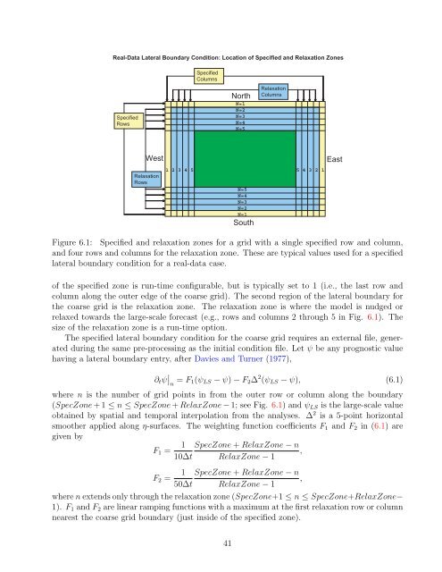
Real-Data Lateral Boundary Condition: Location of Specified and Relaxation Zones
Specified
Rows
West
Relaxation
Rows
Specified
Columns
North
N=1
N=2
N=3
N=4
N=5
1 2 3 4 5 5 4 3 2 1
N=5
N=4
N=3
N=2
N=1
South
Relaxation
Columns
Figure 6.1: Specified and relaxation zones for a grid with a single specified row and column,
and four rows and columns for the relaxation zone. These are typical values used for a specified
lateral boundary condition for a real-data case.
of the specified zone is run-time configurable, but is typically set to 1 (i.e., the last row and
column along the outer edge of the coarse grid). The second region of the lateral boundary for
the coarse grid is the relaxation zone. The relaxation zone is where the model is nudged or
relaxed towards the large-scale forecast (e.g., rows and columns 2 through 5 in Fig. 6.1). The
size of the relaxation zone is a run-time option.
The specified lateral boundary condition for the coarse grid requires an external file, generated
during the same pre-processing as the initial condition file. Let ψ be any prognostic value
having a lateral boundary entry, after Davies and Turner (1977),
East
∂tψ n = F1(ψLS − ψ) − F2∆ 2 (ψLS − ψ), (6.1)
where n is the number of grid points in from the outer row or column along the boundary
(SpecZone + 1 ≤ n ≤ SpecZone + RelaxZone − 1; see Fig. 6.1) and ψLS is the large-scale value
obtained by spatial and temporal interpolation from the analyses. ∆ 2 is a 5-point horizontal
smoother applied along η-surfaces. The weighting function coefficients F1 and F2 in (6.1) are
given by
F1 = 1
10∆t
F2 = 1
50∆t
SpecZone + RelaxZone − n
,
RelaxZone − 1
SpecZone + RelaxZone − n
,
RelaxZone − 1
where n extends only through the relaxation zone (SpecZone+1 ≤ n ≤ SpecZone+RelaxZone−
1). F1 and F2 are linear ramping functions with a maximum at the first relaxation row or column
nearest the coarse grid boundary (just inside of the specified zone).
41