Advanced Research WRF (ARW) Technical Note - MMM - University ...

for Cr > 0, and
(U t q) i+ 1
2
= U t
i+ 1
2
q adv
i+ 1
2
− Cr(q adv
i+ 1
2
− qi+1) + Cr(1 + Cr)(q adv
i+ 1
2
− 2qi+1 + q adv
i+ 3
2
)
(3.54)
for Cr < 0, where Cr = u 1
i+ ∆t/∆x. In addition, to maintain second-order accuracy for the
2
time-split forward-in-time advection scheme, the sequence (3.41) – (3.49) is reversed every other
time step; that is, the flux divergence in η is computed first followed by y and then x. Finally,
the scheme has also been augmented for Courant numbers greater than one using the 1D “semi-
Lagrangian” flux calculation described in Lin and Rood (1996). More information about this
scheme and a description of the limiters can be found in Skamarock (2005).
3.3 Stability Constraints
There are two time steps that a user must specify when running the ARW: the model time step
(the time step used by the RK3 scheme, see Section 3.1.1) and the acoustic time step (used
in the acoustic sub-steps of the time-split integration procedure, see Section 3.1.2). Both are
limited by Courant numbers. In the following sections we describe how to choose time steps for
applications.
3.3.1 RK3 Time Step Constraint
The RK3 time step is limited by the advective Courant number u∆t/∆x and the user’s choice
of advection schemes— users can choose 2 nd through 6 th order discretizations for the advection
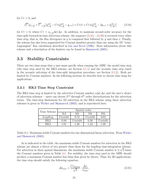
terms. The time-step limitations for 1D advection in the RK3 scheme using these advection
schemes is given in Wicker and Skamarock (2002), and is reproduced here.
Time Scheme
3rd
Spatial order
4th 5th 6th
Leapfrog Unstable 0.72 Unstable 0.62
RK2 0.88 Unstable 0.30 Unstable
RK3 1.61 1.26 1.42 1.08
Table 3.1: Maximum stable Courant numbers for one-dimensional linear advection. From Wicker
and Skamarock (2002).
As is indicated in the table, the maximum stable Courant numbers for advection in the RK3
scheme are almost a factor of two greater than those for the leapfrog time-integration scheme.
For advection in three spatial dimensions, the maximum stable Courant number is 1/ √ 3 times
the Courant numbers given in Table 3.1. For stability, the time step used in the ARW should
produce a maximum Courant number less than that given by theory. Thus, for 3D applications,
the time step should satisfy the following equation:
∆tmax < Crtheory
√
3
21
· ∆x
, (3.55)
umax