EuroSDR Projects - Host Ireland

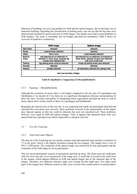
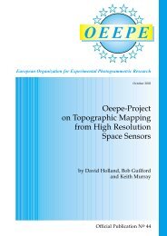
Detection of buildings was not a big problem in SAR and the optical imagery, due to the large size of
industrial buildings. Regarding the classification of parking areas, one can say that the big ones were
detected and classified in optical and even in SAR images. The smaller ones lead to more problems in
SAR imagery. The same is essentially true for bridges and land use boundaries. Table 8 shows an
overview of qualitative comparison.
Main Road
Roads
Alleys
Built-Up
Areas
Parking
Runway
Railway
208
SAR image
detected
predominantly detected
few to none
well detected but no distinction of
industrial or urban areas, separate big
houses were detected well
big parking areas could be detected
detected
partially detected
5.3.3 Summary – Oberpfaffenhofen
land use boundary, bridges
Optical image
detected
detected
predominantly detected
well detected but no distinction of industrial or
urban areas, separate houses were detected
well, even small ones
mostly all parking areas were detected
detected
all interpreters detected the railways well
Table 8: Qualitative Comparison of Oberpfaffenhofen
Although the resolution of sensor data is a bit higher compared to the test sites of Copenhagen and
Fjärdhundra (3 m instead of 4 m), there are no significant discrepancies between interpretations of
these test sites. Accuracy and quality of interpreting forest, agricultural and built-up areas as well as
linear objects show results similar to those in Copenhagen and Fjärdhundra.
Regarding the special areas of this test site, it was surprising that nearly all participants detected and
classified the excavation area correctly. More problems occurred in the interpretation of the airport
area. Special regions on this site could be detected, but were not classified well. These problems,
however, were equal in SAR and optical imagery. Thus, it appears that industrial areas with very
special land uses and objects are almost impossible to interpret correctly.
5.4 Test Site Trudering
5.4.1 Areal and Linear Objects
The data set of the Trudering test site mainly contains rural and industrial areas and has a resolution of
1.5 m per pixel, which is the highest resolution among the test imagery. The images have a size of
2813 x 2289 pixels. The evaluation of the optical image was carried out by four participants and the
evaluation of the SAR image by seven participants.
This test site predominantly consists of agricultural and built-up areas. The forest areas are small parts
with few trees and only cover one percent of the image area. A small lake is located in the north west
of the images, which appears different in SAR and optical images due to the exposure date of the
images. Therefore, two different reference maps were created for this small area. Two other small
parts of the images have different content so they were covered with a small mask to avoid discrepan-