Numerical modeling of waves for a tsunami early warning system
Numerical modeling of waves for a tsunami early warning system
Numerical modeling of waves for a tsunami early warning system

You also want an ePaper? Increase the reach of your titles
YUMPU automatically turns print PDFs into web optimized ePapers that Google loves.
<strong>Numerical</strong> <strong>modeling</strong> <strong>of</strong> <strong>waves</strong> <strong>for</strong> a <strong>tsunami</strong> <strong>early</strong> <strong>warning</strong> <strong>system</strong><br />
The circular shoreline around the conical island has a radius <strong>of</strong> 1m, herea<br />
reflection boundary condition is imposed everywhere, except that in the arc<br />
<strong>of</strong> π/2 posed between θ = −π/4 andθ = π/4. In this arc <strong>of</strong> circumpherence<br />
a wave maker condition is imposed, which introduces a unit source term into<br />
the numerical domain. In the external semi-circumpherence (radius <strong>of</strong> 150m)<br />
a radiation boundary condition is imposed.<br />
The solution <strong>of</strong> the parabolic MSE is obtained using a Crank-Nicolson<br />
finite difference numerical scheme, which proceeds marching towards<br />
increasing values <strong>of</strong> the ray r. The numerical code is written with MatLab<br />
and runs in about 5/10 s on the same computer.<br />
real(A)<br />
abs(A)<br />
angle(A)<br />
0.02<br />
0<br />
−0.02<br />
0.02<br />
0.015<br />
0.01<br />
0.005<br />
4<br />
2<br />
0<br />
−2<br />
θ =0 ◦<br />
80 100 120 140<br />
80 100 120 140<br />
−4<br />
80 100 120 140<br />
r<br />
0.02<br />
0<br />
−0.02<br />
0.02<br />
0.015<br />
0.01<br />
0.005<br />
4<br />
2<br />
0<br />
−2<br />
θ = 180 ◦<br />
80 100 120 140<br />
80 100 120 140<br />
−4<br />
80 100 120 140<br />
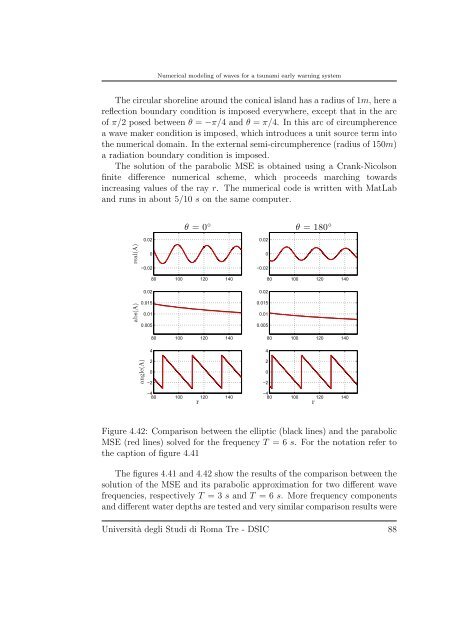
Figure 4.42: Comparison between the elliptic (black lines) and the parabolic<br />
MSE (red lines) solved <strong>for</strong> the frequency T =6s. For the notation refer to<br />
the caption <strong>of</strong> figure 4.41<br />
The figures 4.41 and 4.42 show the results <strong>of</strong> the comparison between the<br />
solution <strong>of</strong> the MSE and its parabolic approximation <strong>for</strong> two different wave<br />
frequencies, respectively T =3s and T =6s. More frequency components<br />
and different water depths are tested and very similar comparison results were<br />
Università degli Studi di Roma Tre - DSIC 88<br />
r