Numerical modeling of waves for a tsunami early warning system

Numerical modeling of waves for a tsunami early warning system
first crest arrives earlier than that measured in the experiments, and the
waves are higher than those expected. Of course the non proper reproduction
of the frequency dispersion leaves all the wave components to propagate
together. As the distance from the generation area grows these errors become
unacceptable.
aFourier
x 10−3
2.5
2
1.5
1
0.5
0
0 10 20 30 40 50 60 70 80
ω (rad/s)
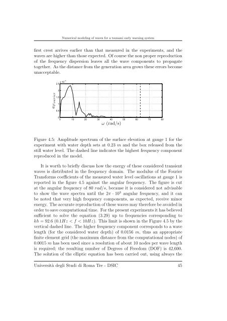
Figure 4.5: Amplitude spectrum of the surface elevation at gauge 1 for the
experiment with water depth sets at 0.23 m and the box released from the
still water level. The dashed line indicates the highest frequency component
reproduced in the model.
It is worth to briefly discuss how the energy of these considered transient
waves is distributed in the frequency domain. The modulus of the Fourier
Transforms coefficients of the measured water level oscillations at gauge 1 is
reported in the figure 4.5 against the angular frequency. The figure is cut
at the angular frequency of 80 rad/s, because it is considered not advisable
to show the wave spectra until the 2π · 10 3 angular frequency, and it can
be noted that very high frequency components, as expected, receive minor
energy. The accurate reproduction of these waves may therefore be avoided in
order to save computational time. For the present experiments it has believed
sufficient to solve the equation (3.29) up to frequencies corresponding to
kh =92.6 (0.1Hz < f < 10Hz). This limit is shown in the Figure 4.5 by the
vertical dashed line. The higher frequency component corresponds to a wave
length (for the considered water depth) of 0.0156 m, thus an appropriate
finite element grid (the maximum distance from the computational nodes) of
0.0015 m has been used since a resolution of about 10 nodes per wave length
is required; the resulting number of Degrees of Freedom (DOF) is 42,600.
The solution of the elliptic equation has been carried out, using always the
Università degli Studi di Roma Tre - DSIC 45