Numerical modeling of waves for a tsunami early warning system

More documents

Recommendations

Info

Numerical modeling of waves for a tsunami early warning system ∇h (gh∇hN)+ω 2 1 N = − cosh (ksh) fft(htt) (4.12) and the model results are compared with the reference solutions of the three dimensional model. η (m) η (m) 0.02 0 −0.02 0.02 0 −0.02 10 15 20 10 15 20 t(s) long landslide 0.02 0 −0.02 short landslide 0.02 0 −0.02 10 15 20 10 15 20 t(s) Figure 4.14: Comparison of the free surface elevation obtained from the three dimensional model (dashed red line) and from the long wave depth integrated model respectively using the frequency filter function (thick black line) and the landslide filter function (thin black line).The presented results are relative to the points A (left panels) and B (right panels) of figure 4.10. Figure 4.14 shows the water surface elevation at point A and B (left and right panels respectively); the top panels refer to the long landslide simulation, while the bottom panel to the short landslide one. With the red dashed lines the three dimensional results are represented, the black lines are relative to the solution of equation (4.11) (thick lines) and equation (4.12) (thin lines). The comparison shows that a smaller extension of the generation area involves, for the landslide filter, a stronger cut in all the frequencies of the wave amplitude. As it can be seen by the thin lines in the bottom panels, these ones do not produce reliable results. The application of the wave frequency filter function better estimates the first crest-trough wave. However some differences arise in the comparison with the three dimensional solutions. These are due to the long wave approximation of the Università degli Studi di Roma Tre - DSIC 59
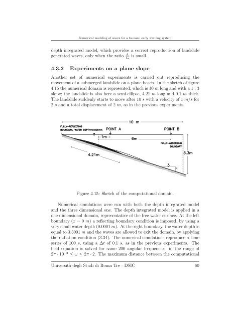
Numerical modeling of waves for a tsunami early warning system depth integrated model, which provides a correct reproduction of landslide generated waves, only when the ratio h is small. Ls 4.3.2 Experiments on a plane slope Another set of numerical experiments is carried out reproducing the movement of a submerged landslide on a plane beach. In the sketch of figure 4.15 the numerical domain is represented, which is 10 m long and with a 1 : 3 slope; the landslide is also here a semi-ellipse, 4.21 m long and 0.1 m thick. The landslide suddenly starts to move after 10 s with a velocity of 1 m/s for 2 s and a total displacement of 2 m, as in the previous experiments. Figure 4.15: Sketch of the computational domain. Numerical simulations were run with both the depth integrated model and the three dimensional one. The depth integrated model is applied in a one-dimensional domain, representative of the free water surface. At the left boundary (x =0m) a reflecting boundary condition is imposed, by using a very small water depth (0.0001 m). At the right boundary, the water depth is equal to 3.3001 m and the waves are allowed to exit the domain, by applying the radiation condition (3.34). The numerical simulations reproduce a time series of 100 s, usingaΔt of 0.1 s, as in the previous experiments. The field equation is solved for same 200 angular frequencies, in the range of 2π · 10 −2 ≤ ω ≤ 2π · 2. The maximum distance between the computational Università degli Studi di Roma Tre - DSIC 60
Page 1 and 2:
Università degli studi ROMA TRE Ph
Page 3 and 4:
To my father Michele, my mother Ant
Page 6 and 7:
Abstract A numerical model based on
Page 8 and 9:
Sommario Un modello numerico basato
Page 10 and 11:
Contents 1 Introduction 3 1.1 Tsuna
Page 12 and 13:
List of Figures 1.1 Principal phase
Page 14 and 15:
xiii 4.13 Panels a and b: absolute
Page 16 and 17:
4.32 Comparison of the free surface
Page 18 and 19:
xvii 5.8 Numerical results of the S
Page 20:
List of Tables 4.1 Radial and Angul
Page 23 and 24:
Numerical modeling of waves for a t
Page 25 and 26:
Page 27 and 28:
Page 29 and 30: Numerical modeling of waves for a t
Page 65 and 66: η1 (m) η2 (m) η3 (m) η4 (m) η5
Page 77 and 78: η (m) 0.02 0 −0.02 Numerical mod
Page 79: aFourier filter functions aFourier
Page 95 and 96: half an hour. ηS12(m) ηS7(m) ηS1
Page 97 and 98: ηS6(m) ηS9(m) Numerical modeling
Page 105 and 106: ηS15(m) ηS24(m) ηS16(m) −0.01
Page 117 and 118: η(m) η(m) η(m) 50 0 Numerical mo
Page 123 and 124: η (m) η (m) η (m) η (m) 20 0
Page 131 and 132:
and Numerical modeling of waves for
Page 133 and 134:
Page 135 and 136:
Page 137 and 138:
Page 139 and 140:
Page 141 and 142:
Page 143 and 144:
Page 145 and 146:
Page 147 and 148:
show all

Numerical modeling of waves for a tsunami early warning system

You also want an ePaper? Increase the reach of your titles

Delete template?

Save as template?