Numerical modeling of waves for a tsunami early warning system

More documents

Recommendations

Info

Numerical modeling of waves for a tsunami early warning system everywhere except in the area where the semi-elliptic landslide moves. At the boundaries (x =0andx =10m) the waves are allowed to exit the domain by imposing the radiation condition specified by the equation (3.34). The simulations here presented reproduce a time series of 100 s, usingaΔt of 0.1 s. This results in a total of 1000 time steps, that in the frequency domain corresponds to the same number of angular frequencies ω, inthe range between 2π · 10 −2 and 2π · 10. In the practice the MSE (4.8) is solved just for the frequencies in the range of 2π · 10 −2 ≤ ω ≤ 2π · 2, where there is a significant content of wave energy. The higher frequency component has, for the considered water depth, a wave length of 0.4 m, thusthemaximum distance between the computational nodes is of 0.04 m, since a resolution of about 10 nodes per wave length is required. The resulting number of Degrees of Freedom (DOF) is 201, and the elliptic equations for the 200 frequencies are solved on a 2 GHz CPU computer equipped with 4 GB of RAM (as all the other simulations presented here), with a total computational time of about 7 s. In the simulations carried out with the three dimensional model, the Laplace equation (4.2) is solved in a two dimensional domain, again 10 m long and 1 m high (as the water depth). At the bottom boundary the condition of wave generation (4.4) is imposed, by letting the landslide to move along the bottom for 2 s. In order to compare the results with those of the depth integrated model, the same angular frequencies ω are solved (2π ·10 −2 ≤ ω ≤ 2π · 2). The finite element grid is composed of linear triangular elements, with the maximum distances between the nodes of 0.04 m, asforthedepth integrated model. The number of DOF for these simulations is 8725 and the computational time is about 53 s. In figure 4.11 the results of the numerical simulations with the two models are shown, in terms of the free surface elevation in time at the points A (left panel) and B (right panel) of figure 4.10. The landslide for the presented simulation is 4 m long and moves between t =10s and t =12s. When the landslide starts moving, going in the direction of increasing x values, it generates a first crest-trough wave propagating in front of it, and a first trough-crest wave at its back. The results computed with the depth integrated model (solid black line) almost perfectly superimpose to the ones obtained from the three dimensional one (dashed red line). The good agreement is both in the generation (left panel) and in the propagation areas (right panel). Simulations with the depth integrated model have been carried out also Università degli Studi di Roma Tre - DSIC 55
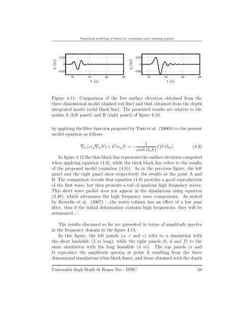
η (m) 0.02 0 −0.02 Numerical modeling of waves for a tsunami early warning system 10 15 20 25 t(s) η (m) 0.02 0 −0.02 10 15 20 25 t(s) Figure 4.11: Comparison of the free surface elevation obtained from the three dimensional model (dashed red line) and that obtained from the depth integrated model (solid black line). The presented results are relative to the points A (left panel) and B (right panel) of figure 4.10. by applying the filter function proposed by Tinti et al. (2006b) to the present model equation as follows ∇h (ccg∇hN)+k 2 1 ccgN = − cosh (ksh) fft(htt) (4.9) In figure 4.12 the thin black line represents the surface elevation computed when applying equation (4.9), while the thick black line refers to the results of the proposed model (equation (4.8)). As in the previous figure, the left panel and the right panel show respectively the results at the point A and B. The comparison reveals that equation (4.9) provides a good reproduction of the first wave, but then presents a tail of spurious high frequency waves. This short wave packet does not appear in the simulations using equation (3.48), which attenuates the high frequency wave components. As stated by Kervella et al. (2007) ‘...the water column has an effect of a low pass filter, thus if the initial deformation contains high frequencies, they will be attenuated...’. The results discussed so far are presented in terms of amplitude spectra in the frequency domain in the figure 4.13. In this figure, the left panels (a, c and e) refer to a simulation with the short landslide (2 m long), while the right panels (b, d and f) tothe same simulation with the long landslide (4 m). The top panels (a and b) reproduce the amplitude spectra at point A resulting from the three dimensional simulations (thin black lines), and those obtained with the depth Università degli Studi di Roma Tre - DSIC 56
Page 1 and 2:
Università degli studi ROMA TRE Ph
Page 3 and 4:
To my father Michele, my mother Ant
Page 6 and 7:
Abstract A numerical model based on
Page 8 and 9:
Sommario Un modello numerico basato
Page 10 and 11:
Contents 1 Introduction 3 1.1 Tsuna
Page 12 and 13:
List of Figures 1.1 Principal phase
Page 14 and 15:
xiii 4.13 Panels a and b: absolute
Page 16 and 17:
4.32 Comparison of the free surface
Page 18 and 19:
xvii 5.8 Numerical results of the S
Page 20:
List of Tables 4.1 Radial and Angul
Page 23 and 24:
Numerical modeling of waves for a t
Page 25 and 26: Numerical modeling of waves for a t
Page 65 and 66: η1 (m) η2 (m) η3 (m) η4 (m) η5
Page 75: Numerical modeling of waves for a t
Page 79 and 80: aFourier filter functions aFourier
Page 95 and 96: half an hour. ηS12(m) ηS7(m) ηS1
Page 97 and 98: ηS6(m) ηS9(m) Numerical modeling
Page 105 and 106: ηS15(m) ηS24(m) ηS16(m) −0.01
Page 117 and 118: η(m) η(m) η(m) 50 0 Numerical mo
Page 123 and 124: η (m) η (m) η (m) η (m) 20 0
Page 127 and 128:
Page 129 and 130:
Page 131 and 132:
and Numerical modeling of waves for
Page 133 and 134:
Page 135 and 136:
Page 137 and 138:
Page 139 and 140:
Page 141 and 142:
Page 143 and 144:
Page 145 and 146:
Page 147 and 148:
show all

Numerical modeling of waves for a tsunami early warning system

Create successful ePaper yourself

Delete template?

Save as template?