Numerical modeling of waves for a tsunami early warning system

Numerical modeling of waves for a tsunami early warning system
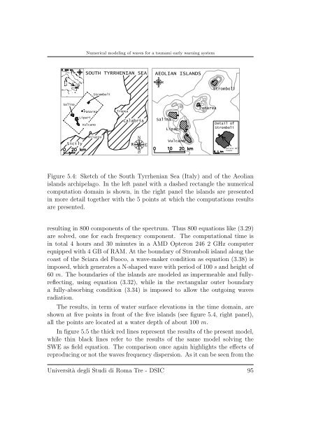
Figure 5.4: Sketch of the South Tyrrhenian Sea (Italy) and of the Aeolian
islands archipelago. In the left panel with a dashed rectangle the numerical
computation domain is shown, in the right panel the islands are presented
in more detail together with the 5 points at which the computations results
are presented.
resulting in 800 components of the spectrum. Thus 800 equations like (3.29)
are solved, one for each frequency component. The computational time is
in total 4 hours and 30 minutes in a AMD Opteron 246 2 GHz computer
equipped with 4 GB of RAM. At the boundary of Stromboli island along the
coast of the Sciara del Fuoco, a wave-maker condition as equation (3.38) is
imposed, which generates a N-shaped wave with period of 100 s and height of
60 m. The boundaries of the islands are modeled as impermeable and fullyreflecting,
using equation (3.32), while in the rectangular outer boundary
a fully-absorbing condition (3.34) is imposed to allow the outgoing waves
radiation.
The results, in term of water surface elevations in the time domain, are
shown at five points in front of the five islands (see figure 5.4, right panel),
all the points are located at a water depth of about 100 m.
In figure 5.5 the thick red lines represent the results of the present model,
while thin black lines refer to the results of the same model solving the
SWE as field equation. The comparison once again highlights the effects of
reproducing or not the waves frequency dispersion. As it can be seen from the
Università degli Studi di Roma Tre - DSIC 95