Asset Pricing John H. Cochrane June 12, 2000

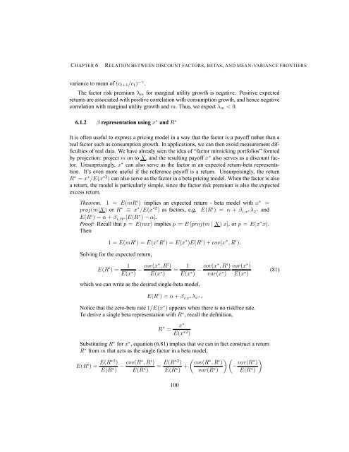
CHAPTER 6 RELATION BETWEEN DISCOUNT FACTORS, BETAS, AND MEAN-VARIANCE FRONTIERS
variance to mean of (ct+1/ct) −γ .
The factor risk premium λm for marginal utility growth is negative. Positive expected
returns are associated with positive correlation with consumption growth, and hence negative
correlation with marginal utility growth and m. Thus, we expect λm < 0.
6.1.2 β representation using x ∗ and R ∗
It is often useful to express a pricing model in a way that the factor is a payoff rather than a
real factor such as consumption growth. In applications, we can then avoid measurement difficulties
of real data. We have already seen the idea of “factor mimicking portfolios” formed
by projection: project m on to X, and the resulting payoff x ∗ also serves as a discount factor.
Unsurprisingly, x ∗ can also serve as the factor in an expected return-beta representation.
It’s even more useful if the reference payoff is a return. Unsurprisingly, the return
R ∗ = x ∗ /E(x ∗2 ) can also serve as the factor in a beta pricing model. When the factor is also
a return, the model is particularly simple, since the factor risk premium is also the expected
excess return.
Theorem. 1 = E(mRi ) implies an expected return - beta model with x∗ =
proj(m|X) or R∗ ≡ x∗ /E(x∗2 ) as factors, e.g. E(Ri ) = α + βi,x∗λx ∗ and
E(Ri )=α + βi,R∗[E(R ∗ ) − α].
Proof: Recall that p = E(mx) implies p = E [proj(m | X) x], orp = E(x∗x). Then
1=E(mR i )=E(x ∗ R i )=E(x ∗ )E(R i )+cov(x ∗ ,R i ).
Solving for the expected return,
E(R i )= 1
E(x∗ ) − cov(x∗ ,Ri )
E(x∗ 1
=
)
which we can write as the desired single-beta model,
E(R i )=α + β i,x ∗λx ∗.
E(x∗ ) − cov(x∗ ,Ri )
var(x∗ )
var(x ∗ )
E(x ∗ )
Notice that the zero-beta rate 1/E(x ∗ ) appears when there is no riskfree rate.
To derive a single beta representation with R ∗ , recall the definition,
R ∗ = x∗
E(x∗2 )
Substituting R∗ for x∗ , equation (6.81) implies that we can in fact construct a return
R∗ from m that acts as the single factor in a beta model,
E(R i )= E(R∗2 )
E(R∗ ) − cov(R∗ ,Ri )
E(R∗ ) = E(R∗2 )
E(R∗ ) +
µ ∗ i cov(R ,R )
var(R∗ µ
−
)
var(R∗ )
E(R∗
)
100
(81)