Asset Pricing John H. Cochrane June 12, 2000

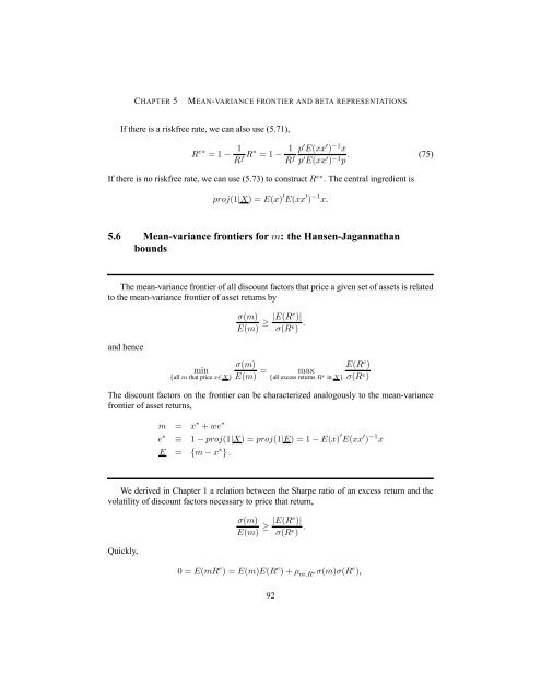
CHAPTER 5 MEAN-VARIANCE FRONTIER AND BETA REPRESENTATIONS
If there is a riskfree rate, we can also use (5.71),
R e∗ =1− 1
R f R∗ =1− 1
R f
p0E(xx0 ) −1x p0E(xx0 ) −1 . (75)
p
If there is no riskfree rate, we can use (5.73) to construct R e∗ . The central ingredient is
proj(1|X) =E(x) 0 E(xx 0 ) −1 x.
5.6 Mean-variance frontiers for m: the Hansen-Jagannathan
bounds
The mean-variance frontier of all discount factors that price a given set of assets is related
to the mean-variance frontier of asset returns by
and hence
σ(m)
E(m) ≥ |E(Re )|
σ(Re ) .
σ(m)
min
= max
{all m that price x∈X} E(m) {all excess returns Re E(R
in X}
e )
σ(Re )
The discount factors on the frontier can be characterized analogously to the mean-variance
frontier of asset returns,
m = x ∗ + we ∗
e ∗ ≡ 1 − proj(1|X) =proj(1|E) =1− E(x) 0 E(xx 0 ) −1 x
E = {m − x ∗ } .
We derived in Chapter 1 a relation between the Sharpe ratio of an excess return and the
volatility of discount factors necessary to price that return,
Quickly,
σ(m)
E(m) ≥ |E(Re )|
σ(Re ) .
0=E(mR e )=E(m)E(R e )+ρ m,R eσ(m)σ(R e ),
92