Asset Pricing John H. Cochrane June 12, 2000

SECTION 4.1 LAW OF ONE PRICE AND EXISTENCE OF A DISCOUNT FACTOR
Theorem: Given free portfolio formation A1, and the law of one price A2, there
exists a unique payoff x ∗ ∈ X such that p(x) =E(x ∗ x) for all x ∈ X.
x∗ is a discount factor. A1 and A2 imply that the price function on X looks like Figure
7: parallel hyperplanes marching out from the origin. The only difference is that X may be a
subspace of the original state space, as shown in Figure 8. The essence of the proof, then, is
that any linear function on a space X can be represented by inner products with a vector that
lies in X.
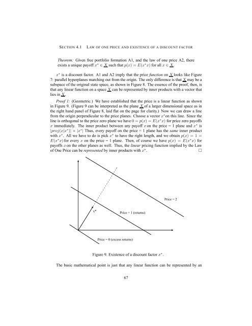
Proof 1: (Geometric.) We have established that the price is a linear function as shown
in Figure 9. (Figure 9 can be interpreted as the plane X of a larger dimensional space as in
the right hand panel of Figure 8, laid flat on the page for clarity.) Now we can draw a line
from the origin perpendicular to the price planes. Choose a vector x∗on this line. Since the
line is orthogonal to the price zero plane we have 0=p(x) =E(x∗x) for price zero payoffs
x immediately. The inner product between any payoff x on the price = 1 plane and x∗ is
|proj(x|x∗ )|×|x∗ | Thus, every payoff on the price = 1 plane has the same inner product
with x∗ . All we have to do is pick x∗ to have the right length, and we obtain p(x) =1=
E(x∗x) for every x on the price = 1 plane. Then, of course we have p(x) =E(x∗x) for
payoffs x on the other planes as well. Thus, the linear pricing function implied by the Law
of One Price can be represented by inner products with x∗ . ¤
x*
Price = 1 (returns)
Price = 0 (excess returns)
Figure 9. Existence of a discount factor x ∗ .
Price = 2
The basic mathematical point is just that any linear function can be represented by an
67