Asset Pricing John H. Cochrane June 12, 2000

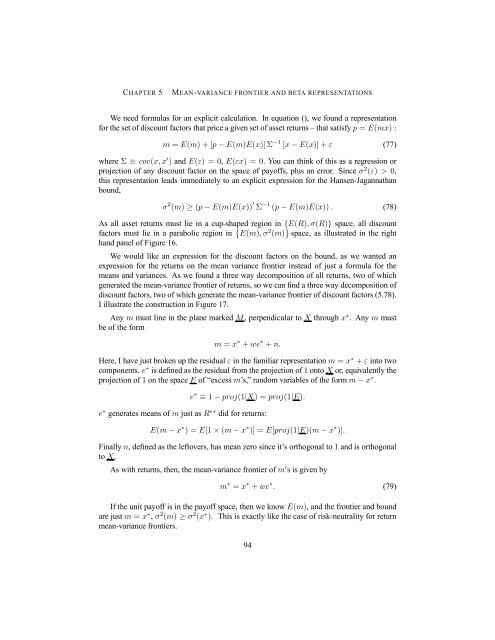
CHAPTER 5 MEAN-VARIANCE FRONTIER AND BETA REPRESENTATIONS
We need formulas for an explicit calculation. In equation (), we found a representation
for the set of discount factors that price a given set of asset returns – that satisfy p = E(mx) :
m = E(m)+[p − E(m)E(x)] Σ −1 [x − E(x)] + ε (77)
where Σ ≡ cov(x, x 0 ) and E(ε) =0, E(εx) =0. You can think of this as a regression or
projection of any discount factor on the space of payoffs, plus an error. Since σ 2 (ε) > 0,
this representation leads immediately to an explicit expression for the Hansen-Jagannathan
bound,
σ 2 (m) ≥ (p − E(m)E(x)) 0 Σ −1 (p − E(m)E(x)) . (78)
As all asset returns must lie in a cup-shaped region in {E(R), σ(R)} space, all discount
factors must lie in a parabolic region in © E(m), σ2 (m) ª space, as illustrated in the right
hand panel of Figure 16.
We would like an expression for the discount factors on the bound, as we wanted an
expression for the returns on the mean variance frontier instead of just a formula for the
means and variances. As we found a three way decomposition of all returns, two of which
generated the mean-variance frontier of returns, so we can find a three way decomposition of
discount factors, two of which generate the mean-variance frontier of discount factors (5.78).
I illustrate the construction in Figure 17.
Any m must line in the plane marked M, perpendicular to X through x∗ .Anymmust be of the form
m = x ∗ + we ∗ + n.
Here, I have just broken up the residual ε in the familiar representation m = x ∗ + ε into two
components. e ∗ is defined as the residual from the projection of 1 onto X or, equivalently the
projection of 1 on the space E of “excess m’s,” random variables of the form m − x ∗ .
e ∗ ≡ 1 − proj(1|X) =proj(1|E).
e ∗ generatesmeansofm just as R e∗ did for returns:
E(m − x ∗ )=E[1 × (m − x ∗ )] = E[proj(1|E)(m − x ∗ )].
Finally n,definedas the leftovers, has mean zero since it’s orthogonal to 1 and is orthogonal
to X.
As with returns, then, the mean-variance frontier of m0sisgivenby m ∗ = x ∗ + we ∗ . (79)
If the unit payoff is in the payoff space, then we know E(m), and the frontier and bound
are just m = x ∗ , σ 2 (m) ≥ σ 2 (x ∗ ). This is exactly like the case of risk-neutrality for return
mean-variance frontiers.
94