Asset Pricing John H. Cochrane June 12, 2000

SECTION 5.6 MEAN-VARIANCE FRONTIERS FOR m: THE HANSEN-JAGANNATHAN BOUNDS
and |ρ| ≤ 1. If we had a riskfree rate, then we know in addition
E(m) =1/R f .
Hansen and Jagannathan (1991) had the brilliant insight to read this equation as a restriction
on the set of discount factors that can price a given set of returns, as well as a restriction on
the set of returns we will see given a specific discount factor. This calculation teaches us
that we need very volatile discount factors with a mean near one to understand stock returns.
This and more general related calculations turn out to be a central tool in understanding and
surmounting the equity premium puzzle, surveyed in Chapter 21.
We would like to derive a bound that uses a large number of assets, and that is valid if
there is no riskfree rate. What is the set of {E(m), σ(m)} consistent with a given set of asset
prices and payoffs? What is the mean-variance frontier for discount factors?
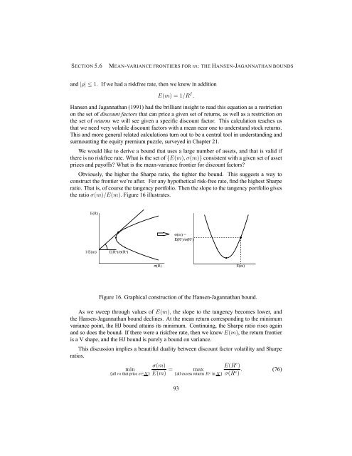
Obviously, the higher the Sharpe ratio, the tighter the bound. This suggests a way to
construct the frontier we’re after. For any hypothetical risk-free rate, find the highest Sharpe
ratio. That is, of course the tangency portfolio. Then the slope to the tangency portfolio gives
the ratio σ(m)/E(m). Figure 16 illustrates.
E(R)
1/E(m) E(R e )/σ(R e )
σ(R)
σ(m) =
Ε(R e )/σ(R e )
E(m)
Figure 16. Graphical construction of the Hansen-Jagannathan bound.
As we sweep through values of E(m), the slope to the tangency becomes lower, and
the Hansen-Jagannathan bound declines. At the mean return corresponding to the minimum
variance point, the HJ bound attains its minimum. Continuing, the Sharpe ratio rises again
and so does the bound. If there were a riskfree rate, then we know E(m), the return frontier
is a V shape, and the HJ bound is purely a bound on variance.
This discussion implies a beautiful duality between discount factor volatility and Sharpe
ratios.
σ(m)
min
= max
{all m that price x∈X} E(m) {all excess returns Re in X}
93
E(Re )
σ(Re . (76)
)