PDF 1.938kB

42 CHAPTER 4. METHOD
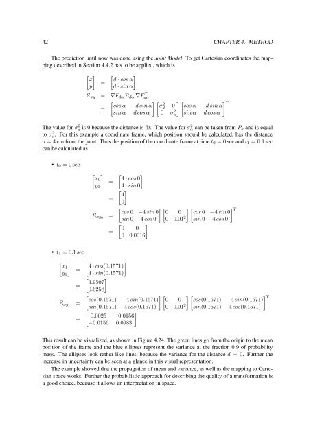
The prediction until now was done using the Joint Model. To get Cartesian coordinates the mapping
described in Section 4.4.2 has to be applied, which is
[ x
y]
=
[ ] d · cos α
d · sin α
Σ xy = ∇F dα Σ dα ∇Fdα
T
[ ] [ ] [ cos α −d sin α σ
2
=
d
0 cos α −d sin α
sin α d cos α 0 σα
2 sin α d cos α
The value for σ 2 d is 0 because the distance is fix. The value for σ2 α can be taken from P k and is equal
to σ 2 s. For this example a coordinate frame, which position should be calculated, has the distance
d = 4 cm from the joint. Thus the position of the coordinate frame at time t 0 = 0 sec and t 1 = 0.1 sec
can be calculated as
] T
• t 0 = 0 sec
[
x0
y 0
]
=
=
[ ] 4 · cos 0
4 · sin 0
[ 4
0]
Σ xy0 =
=
[ ] [ ] [ cos 0 −4 sin 0 0 0 cos 0 −4 sin 0
sin 0 4 cos 0 0 0.01 2 sin 0 4 cos 0
[ ] 0 0
0 0.0016
] T
• t 1 = 0.1 sec
[
x1
y 1
]
=
=
Σ xy1 =
=
[ ]
4 · cos(0.1571)
4 · sin(0.1571)
[ ] 3.9507
0.6258
[ ] [ ] [ cos(0.1571) −4 sin(0.1571) 0 0 cos(0.1571) −4 sin(0.1571)
sin(0.1571) 4 cos(0.1571) 0 0.01 2 sin(0.1571) 4 cos(0.1571)
[ ]
0.0025 −0.0156
−0.0156 0.0983
] T
This result can be visualized, as shown in Figure 4.24. The green lines go from the origin to the mean
position of the frame and the blue ellipses represent the variance at the fraction 0.9 of probability
mass. The ellipses look rather like lines, because the variance for the distance d = 0. Further the
increase in uncertainty can be seen at a glance in this visual representation.
The example showed that the propagation of mean and variance, as well as the mapping to Cartesian
space works. Further the probabilistic approach for describing the quality of a transformation is
a good choice, because it allows an interpretation in space.