PDF 1.938kB

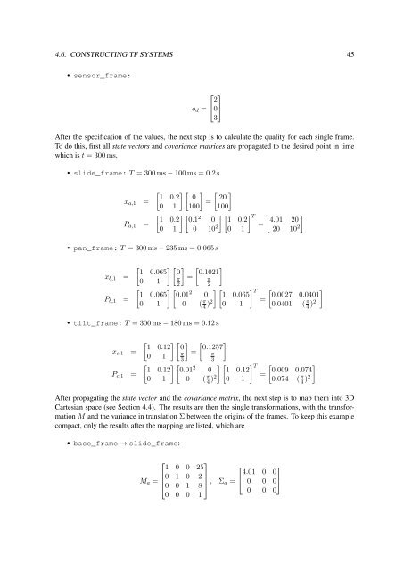
4.6. CONSTRUCTING TF SYSTEMS 45
• sensor_frame:
⎡ ⎤
2
o d = ⎣0⎦
3
After the specification of the values, the next step is to calculate the quality for each single frame.
To do this, first all state vectors and covariance matrices are propagated to the desired point in time
which is t = 300 ms.
• slide_frame: T = 300 ms − 100 ms = 0.2 s
x a,1 =
P a,1 =
[ ] [ ]
1 0.2 0
=
0 1 100
[ 1 0.2
0 1
[ ] 20
100
] [ ] [ 0.1
2
0 1 0.2
0 10 2 0 1
] T
=
[ ] 4.01 20
20 10 2
• pan_frame: T = 300 ms − 235 ms = 0.065 s
x b,1 =
P b,1 =
[ ] [ ]
1 0.065 0
π =
0 1
2
[ 1 0.065
0 1
[ 0.1021
π
2
] [ 0.01
2
0
0 ( π 4 )2 ] [ 1 0.065
0 1
]
] T
=
[ ]
0.0027 0.0401
0.0401 ( π 4 )2
• tilt_frame: T = 300 ms − 180 ms = 0.12 s
x c,1 =
P c,1 =
[ ] [ ]
1 0.12 0
π =
0 1
3
[ 1 0.12
0 1
[ 0.1257
π
] [ 0.01
2
0
0 ( π 4 )2 ] [ 1 0.12
0 1
3
]
] T
=
[ ]
0.009 0.074
0.074 ( π 4 )2
After propagating the state vector and the covariance matrix, the next step is to map them into 3D
Cartesian space (see Section 4.4). The results are then the single transformations, with the transformation
M and the variance in translation Σ between the origins of the frames. To keep this example
compact, only the results after the mapping are listed, which are
• base_frame → slide_frame:
⎡
⎤
1 0 0 25 ⎡ ⎤
M a = ⎢0 1 0 2
4.01 0 0
⎥
⎣0 0 1 8 ⎦ , Σ a = ⎣ 0 0 0⎦
0 0 0
0 0 0 1