Modelling Dependence with Copulas - IFOR

5 Archimedean Copulas
In this chapter we discuss an important class of copulas called Archimedean copulas.
This class of copulas is worth studying for a number of reasons: 1) The many
parametric families of copulas belonging to this class 2) The great variety of different
dependence structures 3) The many nice properties possessed by members of this
class 4) The ease with which they can be constructed and simulated from. At the
end of this chapter we present one possible multivariate extension of Archimedean
copulas and a general algorithm for random variate generation for those families of
n-copulas. For other multivariate extensions we refer to Joe (1997) [6].
5.1 Convex Sums
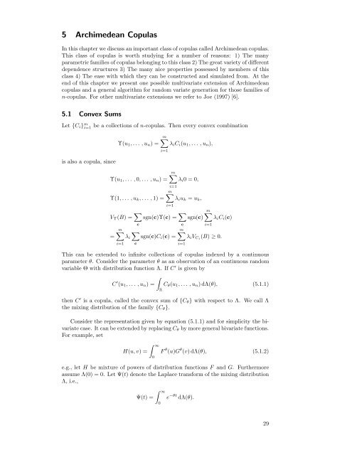
Let {C i } m i=1 be a collections of n-copulas. Then every convex combination
is also a copula, since
Υ(u 1 ,... ,u n )=
m∑
λ i C i (u 1 ,... ,u n ),
i=1
Υ(u 1 ,... ,0,... ,u n )=
Υ(1,... ,u k ,... ,1) =
m∑
λ i 0=0,
i=1
m∑
λ i u k = u k ,
i=1
V Υ (B) = ∑ sgn(c)Υ(c) = ∑ m∑
sgn(c) λ i C i (c)
c
c
i=1
m∑ ∑
m∑
= λ i sgn(c)C i (c) = λ i V Ci (B) ≥ 0.
i=1
c
This can be extended to infinite collections of copulas indexed by a continuous
parameter θ. Consider the parameter θ as an observation of an continuous random
variable Θ with distribution function Λ. If C ′ is given by
∫
C ′ (u 1 ,... ,u n )= C θ (u 1 ,... ,u n )dΛ(θ), (5.1.1)
R
then C ′ is a copula, called the convex sum of {C θ } with respect to Λ. We call Λ
the mixing distribution of the family {C θ }.
Consider the representation given by equation (5.1.1) and for simplicity the bivariate
case. It can be extended by replacing C θ by more general bivariate functions.
For example, set
H(u, v) =
∫ ∞
0
i=1
F θ (u)G θ (v)dΛ(θ), (5.1.2)
e.g., let H be mixture of powers of distribution functions F and G. Furthermore
assume Λ(0) = 0. Let Ψ(t) denote the Laplace transform of the mixing distribution
Λ, i.e.,
Ψ(t) =
∫ ∞
0
e −θt dΛ(θ).
29