

Modelling Dependence with Copulas - IFOR
Modelling Dependence with Copulas - IFOR
Modelling Dependence with Copulas - IFOR

Create successful ePaper yourself
Turn your PDF publications into a flip-book with our unique Google optimized e-Paper software.
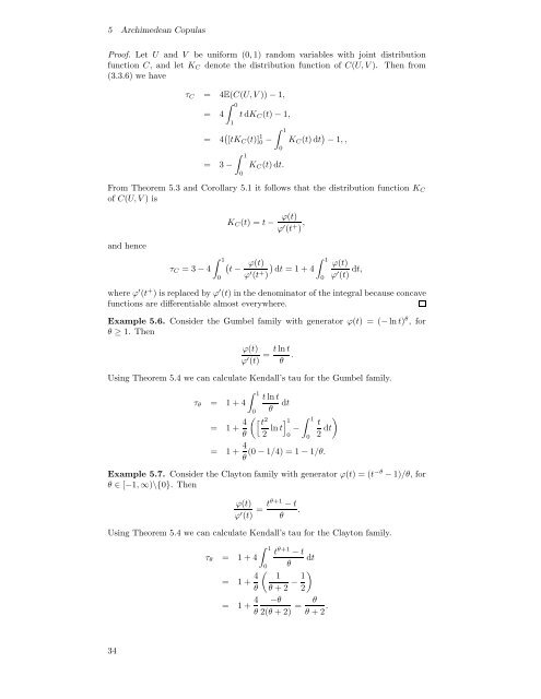
5 Archimedean <strong>Copulas</strong><br />
Proof. Let U and V be uniform (0, 1) random variables <strong>with</strong> joint distribution<br />
function C, and let K C denote the distribution function of C(U, V ). Then from<br />
(3.3.6) we have<br />
τ C = 4E(C(U, V )) − 1,<br />
= 4<br />
∫ 0<br />
1<br />
t dK C (t) − 1,<br />
= 4 ( [tK C (t)] 1 0 −<br />
= 3−<br />
∫ 1<br />
0<br />
∫ 1<br />
0<br />
K C (t)dt.<br />
K C (t)dt ) − 1,,<br />
From Theorem 5.3 and Corollary 5.1 it follows that the distribution function K C<br />
of C(U, V )is<br />
and hence<br />
τ C =3− 4<br />
∫ 1<br />
0<br />
K C (t) =t −<br />
(<br />
t −<br />
ϕ(t)<br />
ϕ ′ (t + )<br />
ϕ(t)<br />
ϕ ′ (t + ) ,<br />
)<br />
dt =1+4<br />
∫ 1<br />
0<br />
ϕ(t)<br />
ϕ ′ (t) dt,<br />
where ϕ ′ (t + ) is replaced by ϕ ′ (t) in the denominator of the integral because concave<br />
functions are differentiable almost everywhere.<br />
Example 5.6. Consider the Gumbel family <strong>with</strong> generator ϕ(t) =(− ln t) θ ,for<br />
θ ≥ 1. Then<br />
ϕ(t)<br />
ϕ ′ (t) = t ln t<br />
θ .<br />
Using Theorem 5.4 we can calculate Kendall’s tau for the Gumbel family.<br />
∫ 1<br />
t ln t<br />
τ θ = 1+4 dt<br />
0 θ<br />
= 1+ 4 ( [t 2 ] 1<br />
∫ 1<br />
)<br />
θ 2 ln t t<br />
−<br />
0 0 2 dt<br />
= 1+ 4 (0 − 1/4) = 1 − 1/θ.<br />
θ<br />
Example 5.7. Consider the Clayton family <strong>with</strong> generator ϕ(t) =(t −θ − 1)/θ, for<br />
θ ∈ [−1, ∞)\{0}. Then<br />
ϕ(t)<br />
ϕ ′ (t) = tθ+1 − t<br />
.<br />
θ<br />
Using Theorem 5.4 we can calculate Kendall’s tau for the Clayton family.<br />
∫ 1<br />
t θ+1 − t<br />
τ θ = 1+4<br />
dt<br />
0 θ<br />
= 1+ 4 ( 1<br />
θ θ +2 − 1 )<br />
2<br />
= 1+ 4 −θ<br />
θ 2(θ +2) = θ<br />
θ +2 .<br />
34


