Modelling Dependence with Copulas - IFOR
Modelling Dependence with Copulas - IFOR
Modelling Dependence with Copulas - IFOR
You also want an ePaper? Increase the reach of your titles
YUMPU automatically turns print PDFs into web optimized ePapers that Google loves.
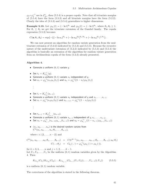
5.5 Multivariate Archimedean <strong>Copulas</strong><br />
ϕ 2 ◦ ϕ −1<br />
3 are in L ∗ ∞ , then (5.5.4) is a proper copula. Note that all trivariate margins<br />
of (5.5.4) have the form (5.5.3) and all bivariate margins have the form (5.2.2).<br />
Clearly the idea of (5.5.3) and (5.5.4) generalizes to higher dimensions.<br />
Example 5.13. Let ϕ θ1 (t) =(− ln t) θ1 and ϕ θ2 (t) =(− ln t) θ2 ,whereθ 1 ,θ 2 ≥ 1.<br />
For θ 1 ≤ θ 2 we get the trivariate extension of the Gumbel family. The copula<br />
expression (5.5.3) becomes<br />
C(u; θ 1 ,θ 2 )=exp{−([(− ln u 1 ) θ2 +(− ln u 2 ) θ2 ] θ1/θ2 +(− ln u 3 ) θ1 ) 1/θ1 }.<br />
We can now present an algorithm for random variate generation from the multivariate<br />
extension of (5.2.2) indicated by (5.5.3) and (5.5.4). Because the recursive<br />
nature of the multivariate extension of (5.2.2) indicated by (5.5.3) and (5.5.4) the<br />
algorithm is basically an extension of the algorithm for random variate generation<br />
from an Archimedean copula of the form (5.2.2) already presented.<br />
Algorithm 4.<br />
• Generate a uniform (0, 1) variate q.<br />
• Set t 1 = K −1<br />
C θ1<br />
(q).<br />
• Generate a uniform (0, 1) variate s 1 independent of q.<br />
• Set a 1 = ϕ −1<br />
θ 1<br />
(s 1 ϕ θ1 (t 1 )) and u n = ϕ −1<br />
θ 1<br />
((1 − s 1 )ϕ θ1 (t 1 ))<br />
.<br />
.<br />
• Set t i = K −1<br />
C θi<br />
(a i−1 ).<br />
• Generate a uniform (0, 1) variate s k independent of q and s 1 ,... ,s i−1 .<br />
• Set a i = ϕ −1<br />
θ i<br />
.<br />
(s i ϕ θi (t k )) and u n−i+1 = ϕ −1<br />
θ i<br />
((1 − s i )ϕ θi (t i ))<br />
• Set t n−1 = K −1<br />
C θn−1<br />
(a n−2 ).<br />
• Generate a uniform (0, 1) variate s n−1 independent of q, s 1 ,... ,s n−2 .<br />
• Set u 1 = ϕ −1<br />
θ n−1<br />
(s n−1 ϕ θn−1 (t n−1 )) and u 2 = ϕ −1<br />
θ n−1<br />
((1 − s n−1 )ϕ θn−1 (t n−1 ))<br />
• (u 1 ,u 2 ,... ,u n ) is the desired random variate from<br />
C n (u 1 ,u 2 ,... ,u n ; θ 1 ,... ,θ n−1 ),<br />
where i ∈{2,... ,n− 2} and<br />
C k (u 1 ,u 2 ,... ,u k ; θ 1 ,... ,θ k−1 ) = C(C k−1 (u 1 ,u 2 ,... ,u k−1 ; θ 2 ,... ,θ k−1 ),u k ; θ 1 )<br />
C(·, ·; θ j ) = C θj (·, ·) =ϕ −1<br />
θ j<br />
(ϕ θj (·)+ϕ θj (·)),<br />
for k =3, 4,... ,n and j =1, 2,... ,k− 1.<br />
Let U 1 ,U 2 ,... ,U n be the uniform (0, 1) random variables given by the Algorithm<br />
4. Then<br />
K Cθ1 (C θ1 (K Cθ2 (C θ2 (...K Cθn−1 (C θn−1 (U 1 ,U 2 )),... ,U n−1 )),U n )) (5.5.5)<br />
is a uniform (0, 1) random variable.<br />
The correctness of the algorithm is stated in the following theorem.<br />
41


