Modelling Dependence with Copulas - IFOR
Modelling Dependence with Copulas - IFOR
Modelling Dependence with Copulas - IFOR
Create successful ePaper yourself
Turn your PDF publications into a flip-book with our unique Google optimized e-Paper software.
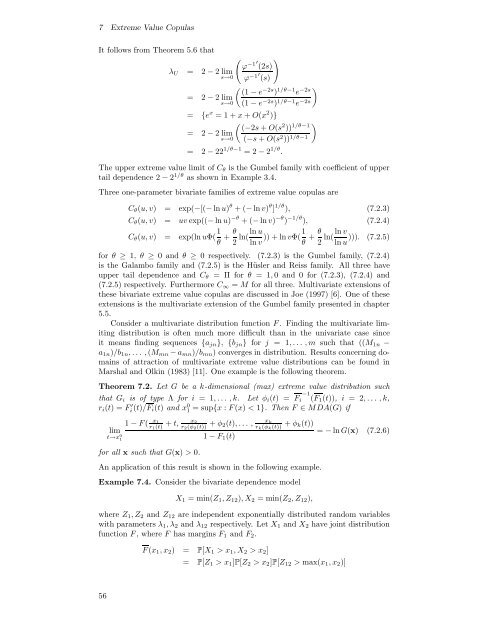
7 Extreme Value <strong>Copulas</strong><br />
It follows from Theorem 5.6 that<br />
λ U =<br />
( )<br />
ϕ −1′ (2s)<br />
2− 2 lim<br />
s→0 ϕ −1′ (s)<br />
=<br />
( (1 − e −2s ) 1/θ−1 e −2s )<br />
2− 2 lim<br />
s→0 (1 − e −2s ) 1/θ−1 e −2s<br />
= {e x =1+x + O(x 2 )}<br />
( (−2s + O(s 2 )) 1/θ−1 )<br />
= 2− 2 lim<br />
s→0 (−s + O(s 2 )) 1/θ−1<br />
= 2− 22 1/θ−1 =2− 2 1/θ .<br />
The upper extreme value limit of C θ is the Gumbel family <strong>with</strong> coefficient of upper<br />
tail dependence 2 − 2 1/θ as shown in Example 3.4.<br />
Three one-parameter bivariate families of extreme value copulas are<br />
C θ (u, v) = exp(−[(− ln u) θ +(− ln v) θ ] 1/θ ), (7.2.3)<br />
C θ (u, v) = uv exp((− ln u) −θ +(− ln v) −θ ) −1/θ ), (7.2.4)<br />
C θ (u, v) = exp(ln uΦ( 1 θ + θ 2 ln(ln u<br />
ln v )) + ln vΦ(1 θ + θ ln v<br />
ln( ))). (7.2.5)<br />
2 ln u<br />
for θ ≥ 1, θ ≥ 0andθ ≥ 0 respectively. (7.2.3) is the Gumbel family, (7.2.4)<br />
is the Galambo family and (7.2.5) is the Hüsler and Reiss family. All three have<br />
upper tail dependence and C θ = Π for θ = 1, 0 and 0 for (7.2.3), (7.2.4) and<br />
(7.2.5) respectively. Furthermore C ∞ = M for all three. Multivariate extensions of<br />
these bivariate extreme value copulas are discussed in Joe (1997) [6]. One of these<br />
extensions is the multivariate extension of the Gumbel family presented in chapter<br />
5.5.<br />
Consider a multivariate distribution function F . Finding the multivariate limiting<br />
distribution is often much more difficult than in the univariate case since<br />
it means finding sequences {a jn }, {b jn } for j = 1,... ,m such that ((M 1n −<br />
a 1n )/b 1n ,... ,(M mn − a mn )/b mn ) converges in distribution. Results concerning domains<br />
of attraction of multivariate extreme value distributions can be found in<br />
Marshal and Olkin (1983) [11]. One example is the following theorem.<br />
Theorem 7.2. Let G be a k-dimensional (max) extreme value distribution such<br />
−1<br />
that G i is of type Λ for i = 1,... ,k. Let φ i (t) = F i (F1 (t)), i = 2,... ,k,<br />
r i (t) =F i ′(t)/F<br />
i(t) and x 0 1 =sup{x : F (x) < 1}. Then F ∈ MDA(G) if<br />
1 − F ( x1<br />
r<br />
lim<br />
+ t, x 2<br />
1(t)<br />
t→x 0 1<br />
for all x such that G(x) > 0.<br />
r + φ 2(φ 2(t)) 2(t),... ,<br />
1 − F 1 (t)<br />
x k<br />
r k (φ k (t)) + φ k(t))<br />
An application of this result is shown in the following example.<br />
Example 7.4. Consider the bivariate dependence model<br />
X 1 = min(Z 1 ,Z 12 ),X 2 =min(Z 2 ,Z 12 ),<br />
= − ln G(x) (7.2.6)<br />
where Z 1 ,Z 2 and Z 12 are independent exponentially distributed random variables<br />
<strong>with</strong> parameters λ 1 ,λ 2 and λ 12 respectively. Let X 1 and X 2 have joint distribution<br />
function F ,whereF has margins F 1 and F 2 .<br />
F (x 1 ,x 2 ) = P[X 1 >x 1 ,X 2 >x 2 ]<br />
= P[Z 1 >x 1 ]P[Z 2 >x 2 ]P[Z 12 > max(x 1 ,x 2 )]<br />
56


