Modelling Dependence with Copulas - IFOR

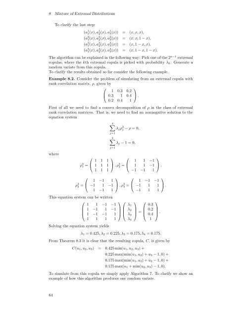
8 Mixture of Extremal Distributions
To clarify the last step:
(a 1 1 (x),a1 2 (x),a1 3 (x)) = (x, x, x),
(a 2 1 (x),a2 2 (x),a2 3 (x)) = (x, x, 1 − x),
(a 3 1(x),a 3 2(x),a 3 3(x)) = (x, 1 − x, x),
(a 4 1 (x),a4 2 (x),a4 3 (x)) = (x, 1 − x, 1 − x).
The algorithm can be explained in the following way: Pick one of the 2 n−1 extremal
copulas, where the kth extremal copula is picked with probability λ k . Generate a
random variate from this copula.
To clarify the results obtained so far consider the following example.
Example 8.2. Consider the problem of simulating from an extremal copula with
rank correlation matrix, ρ, givenby
⎛
⎞
1 0.3 0.2
⎝ 0.3 1 0.4 ⎠ .
0.2 0.4 1
First of all we need to find a convex decomposition of ρ in the class of extremal
rank correlation matrices. That is, we need to find an nonnegative solution to the
equation system
4∑
λ j ρ 3 j − ρ =0,
where
j=1
4∑
λ j − 1=0,
j=1
⎛
ρ 3 1 = ⎝ 1 1 1 ⎞ ⎛
1 1 1 ⎠ ,ρ 3 2 = ⎝ 1 1 −1 ⎞
1 1 −1 ⎠ ,
1 1 1
−1 −1 1
⎛
ρ 3 3 = ⎝ 1 −1 1 ⎞ ⎛
−1 1 −1 ⎠ ,ρ 3 4 = ⎝
1 −1 1
This equation system can be written
⎛
⎞ ⎛ ⎞ ⎛
1 1 −1 −1 λ 1
⎜ 1 −1 1 −1
⎟ ⎜ λ 2
⎟
⎝ 1 −1 −1 1 ⎠ ⎝ λ 3
⎠ = ⎜
⎝
1 1 1 1 λ 4
Solving the equation system yields
1 −1 −1
−1 1 1
−1 1 1
0.3
0.2
0.4
1
⎞
⎟
⎠ .
λ 1 =0.425,λ 2 =0.225,λ 3 =0.175,λ 4 =0.175.
⎞
⎠ .
From Theorem 8.3 it is clear that the resulting copula, C, isgivenby
C(u 1 ,u 2 ,u 3 ) = 0.425 min(u 1 ,u 2 ,u 3 )+
0.225 max(min(u 1 ,u 2 )+u 3 − 1, 0) +
0.175 max(min(u 1 ,u 3 )+u 2 − 1, 0) +
0.175 max(u 1 + min(u 2 ,u 3 ) − 1, 0).
To simulate from this copula we simply apply Algorithm 7. To clarify we show an
example of how this algorithm produces one random variate.
64