Modelling Dependence with Copulas - IFOR

9.2 The Perfect Storm
100
90
80
70
Expected Shortfall
60
50
40
30
20
10
0
0 5 10 15 20 25 30 35 40 45 50
Threshold
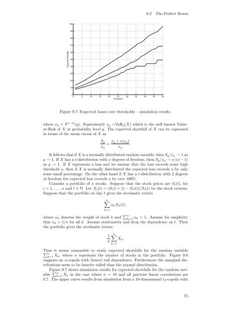
Figure 9.7: Expected losses over thresholds – simulation results.
where x q = F (−1) (q). Equivalently x q =VaR q (X) which is the well known Valueat-Risk
of X at probability level q. The expected shortfall of X can be expressed
in terms of the mean excess of X as
S q
= x q + e(x q )
.
x q x q
It follows that if X is a normally distributed random variable, then S q /x q → 1as
q → 1. If X has a t-distribution with ν degrees of freedom, then S q /x q → ν/(ν − 1)
as q → 1. If X represents a loss and we assume that the loss exceeds some high
threshold u, thenifX is normally distributed the expected loss exceeds u by only
some small percentage. On the other hand if X has a t-distribution with 2 degrees
of freedom the expected loss exceeds u by over 100%.
Consider a portfolio of n stocks. Suppose that the stock prices are S i (t), for
i =1,... ,n and t ∈ N. Let X i (t) =(S i (t +1)− S i (t))/S i (t) be the stock returns.
Suppose that the portfolio on day t gives the stochastic return
n∑
α k X k (t),
k=1
where α k denotes the weight of stock k and ∑ n
k=1 α k = 1. Assume for simplicity
that α k =1/n for all k. Assume stationarity and drop the dependence on t. Then
the portfolio gives the stochastic return
1
n
n∑
X k .
k=1
Thus
∑
it seems reasonable to study expected shortfalls for the random variable
n
k=1 X k,wheren represents the number of stocks in the portfolio. Figure 9.6
suggests an n-copula with (lower) tail dependence. Furthermore the marginal distributions
seem to be heavier tailed than the normal distribution.
Figure 9.7 shows simulation results for expected shortfalls for the random variable
∑ n
k=1 X k in the case where n = 10 and all pairwise linear correlations are
0.7. The upper curve results from simulation from a 10-dimensional t 2 -copula with
75