Modelling Dependence with Copulas - IFOR
Modelling Dependence with Copulas - IFOR
Modelling Dependence with Copulas - IFOR
You also want an ePaper? Increase the reach of your titles
YUMPU automatically turns print PDFs into web optimized ePapers that Google loves.
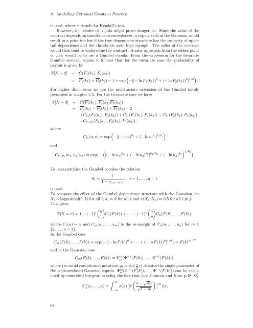
9 <strong>Modelling</strong> Extremal Events in Practice<br />
is used, where τ stands for Kendall’s tau.<br />
However, this choice of copula might prove dangerous. Since the value of the<br />
contract depends on simultaneous exceedences, a copula such as the Gaussian would<br />
result in a price too low if the true dependence structure has the property of upper<br />
tail dependence and the thresholds were high enough. The seller of the contract<br />
would then tend to undervalue the contract. A safer approach from the sellers point<br />
of view would be to use a Gumbel copula. From the expression for the bivariate<br />
Gumbel survival copula it follows that for the bivariate case the probability of<br />
payout is given by<br />
P[N =2] = Ĉ(F 1(k 1 ), F 2 (k 2 ))<br />
(<br />
= F 1 (k 1 )+F 2 (k 2 ) − 1+exp −[(− ln F 1 (k 1 )) θ +(− ln F 2 (k 2 )) θ ] 1/θ) .<br />
For higher dimensions we use the multivariate extension of the Gumbel family<br />
presented in chapter 5.5. For the trivariate case we have<br />
P[N =3] = Ĉ(F 1(k 1 ), F 2 (k 2 )F 3 (k 3 ))<br />
= F 1 (k 1 )+F 2 (k 2 )+F 3 (k 3 ) − 2<br />
+C θ2 (F 1 (k 1 ),F 2 (k 2 )) + C θ1 (F 1 (k 1 ),F 3 (k 3 )) + C θ1 (F 2 (k 2 ),F 3 (k 3 ))<br />
−C θ1,θ 2<br />
(F 1 (k 1 ),F 2 (k 2 ),F 3 (k 3 )),<br />
where<br />
and<br />
C θ1,θ 2<br />
(u 1 ,u 2 ,u 3 )=exp{−<br />
)<br />
C θi (u, v) =exp<br />
(−[(− ln u) θi +(− ln v) θi ] 1/θi<br />
(<br />
[(− ln u 1 ) θ2 +(− ln u 2 ) θ2 ] θ1/θ2 +(− ln u 3 ) θ1 ) 1/θ1}.<br />
To parametrizise the Gumbel copulas the relation<br />
1<br />
θ i =<br />
, i =1,...,n− 1<br />
1 − τ 1,n−i+1<br />
is used.<br />
To compare the effect of the Gumbel dependence structure <strong>with</strong> the Gaussian, let<br />
X i ∼Lognormal(0, 1) for all i, k i = k for all i and τ(X i ,X j )=0.5 for all i ≠ j.<br />
This gives<br />
( )<br />
( )<br />
n n<br />
P[N = n] =1+(−1) 1 C 1 (F (k)) + ···+(−1) n C n (F (k),...,F(k)),<br />
1<br />
n<br />
where C 1 (u) =u and C m (u 1 ,...,u m )isthem-margin of C n (u 1 ,...,u n )form ∈<br />
{2,...,n− 1}.<br />
In the Gumbel case<br />
C m (F (k),...,F(k)) = exp{−[(− ln F (k)) θ + ···+(− ln F (k)) θ ] 1/θ } = F (k) m1/θ<br />
and in the Gaussian case<br />
C m (F (k),...,F(k)) = Φ m ρ l<br />
(Φ −1 (F (k)),...,Φ −1 (F (k))),<br />
where (to avoid complicated notation) ρ l = sin( π 2<br />
τ) denotes the single parameter of<br />
the equicorrelated Gaussian copula. Φ m ρ l<br />
(Φ −1 (F (k)),...,Φ −1 (F (k))) can be calculated<br />
by numerical integration using the fact that (see Johnson and Kotz p.48 [8])<br />
∫ ∞<br />
Φ m ρ l<br />
(a,...,a)= φ(x) [ ( √ ) a − ρl x ]m<br />
Φ √ dx,<br />
1 − ρl<br />
−∞<br />
68


