Rural Development Policies and Sustainable Land Use in the ...

More documents

Recommendations

Info

52 CHAPTER 5 The socioeconomic explanatory variables included in the model represent households’ human capital and geographic determinants of comparative advantage. As explained in Chapter 3, we decided not to include other types of capital because of concerns that these may be endogenous to the choice of livelihood strategy. Geographic determinants of comparative advantage are represented by population density, market access, and road density. Following Pender, Scherr, and Durón (2001), we expect population density to influence both crop choice and production technologies. Whereas improved market access can be expected to stimulate production of cash crops, the effect on adoption of conservation practices is often ambiguous (Pender et al. 2004). Higher road densities tend to lead to improved market access and are expected to stimulate cash crops. Moreover, better road connections are expected to facilitate off-farm work. Human capital variables in the model include household size, dependency ratio, gender and age of the household head, proportion of adults in the household who are female, and the median education of household members. Size of the household determines the availability of family labor and as such is expected to influence both livelihood strategy and technology use. For example, to maximize employment for its members, large households may want to adopt a livelihood strategy that centers on working on the own farms. They may also find it easier to adopt labor-intensive production technologies. On the other hand, a high dependency ratio may be indicative of labor scarcity, which may stimulate livelihood strategies that require less family labor. Given a number of specific characteristics of femaleheaded households and the many competing demands on the time of female household heads (see Box 4.2 in Chapter 4), gender of the household head is expected to influence the choice of livelihood strategy. A higher proportion of female adults in the household decreases the availability of non-domestic labor (the fact that most female adults have children restricts their options for nondomestic work) and therefore may influence the household’s choice of livelihood strategy as well as technology choice. Finally, households in which the average level of education is higher can be expected to have more members working off-farm (often in better remunerated occupations) and be more receptive to new technologies. The results of our multinomial logit model are presented in Table 5.1. The coefficients represent the effect of each explanatory variable on the ratio of the probability of the household selecting the particular livelihood strategy considered, relative to the probability of selecting the basic grains only strategy. 42 In general terms the results suggest that livelihood strategies are associated with differences in both biophysical conditions (natural assets) and socioeconomic conditions (human assets and geographic determinants of comparative advantage) that jointly determine the way in which an individual household puts these assets to use. Note that there is little difference between the mean proportions of each cluster and the mean predicted probabilities of each cluster, indicating good fit of the model to the data. To ease interpretation of the model results, we report the marginal effects of the 42 More precisely, the coefficient of a particular explanatory variable represents the impact of a unit change in that variable on the natural logarithm of the ratio of probabilities (“odds ratio”) of the strategy represented by the particular column of the table, relative to the basic grains strategy. By exponentiating the coefficients, we can find the impact of the variables on the odds ratio. For example, the coefficient of –3.965 for the effect of female household head on the coffee producer strategy means that the odds ratio of choosing the coffee relative to the basic grains strategy for a female-headed household is less than 2 percent (e –3.965 = 0.019) of the odds ratio for a maleheaded household. For any coefficients less than zero, the explanatory variable reduces the odds ratio, while for any coefficients greater than zero, the variable increases the odds ratio.
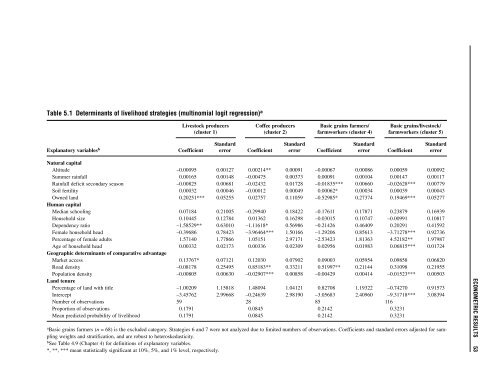
Table 5.1 Determinants of livelihood strategies (multinomial logit regression) a Livestock producers Coffee producers Basic grains farmers/ Basic grains/livestock/ (cluster 1) (cluster 2) farmworkers (cluster 4) farmworkers (cluster 5) Standard Standard Standard Standard Explanatory variables b Coefficient error Coefficient error Coefficient error Coefficient error Natural capital Altitude –0.00095 0.00127 0.00214** 0.00091 –0.00067 0.00086 0.00059 0.00092 Summer rainfall 0.00165 0.00148 –0.00475 0.00373 0.00091 0.00104 0.00147 0.00117 Rainfall deficit secondary season –0.00825 0.00681 –0.02432 0.01728 –0.01835*** 0.00660 –0.02628*** 0.00779 Soil fertility 0.00032 0.00046 –0.00012 0.00049 0.00062* 0.00034 0.00039 0.00043 Owned land 0.20251*** 0.05255 0.02757 0.11059 –0.52985* 0.27374 0.19469*** 0.05277 Human capital Median schooling 0.07184 0.21005 –0.29940 0.18422 –0.17611 0.17871 0.23879 0.16939 Household size 0.10445 0.12784 0.01362 0.16298 –0.03015 0.10747 –0.00991 0.10817 Dependency ratio –1.58529** 0.63010 –1.11618* 0.56986 –0.21426 0.46409 0.20291 0.41592 Female household head –0.39686 0.78423 –3.96464*** 1.50166 –1.29206 0.85613 –3.71278*** 0.92736 Percentage of female adults 1.57140 1.77866 1.05151 2.97171 –2.53423 1.81363 4.52182** 1.97987 Age of household head 0.00332 0.02173 0.00336 0.02309 0.02956 0.01983 0.06815*** 0.01724 Geographic determinants of comparative advantage Market access 0.13767* 0.07121 0.12030 0.07902 0.09003 0.05954 0.09858 0.06820 Road density –0.08178 0.25495 0.85183** 0.33211 0.51997** 0.21144 0.31098 0.21955 Population density –0.00805 0.00630 –0.02907*** 0.00858 –0.00429 0.00414 –0.01523*** 0.00503 Land tenure Percentage of land with title –1.00209 1.15818 1.48094 1.04121 0.82708 1.19322 –0.74270 0.91573 Intercept –3.45762 2.99668 –0.24639 2.98190 –3.05683 2.40960 –9.31718*** 3.08394 Number of observations 59 28 85 116 Proportion of observations 0.1791 0.0845 0.2142 0.3231 Mean predicted probability of livelihood 0.1791 0.0845 0.2142 0.3231 a Basic grains farmers (n = 68) is the excluded category. Strategies 6 and 7 were not analyzed due to limited numbers of observations. Coefficients and standard errors adjusted for sampling weights and stratification, and are robust to heteroskedasticity. b See Table 4.9 (Chapter 4) for definitions of explanatory variables. *, **, *** mean statistically significant at 10%, 5%, and 1% level, respectively. ECONOMETRIC RESULTS 53
Page 1 and 2:
Rural Development Policies and Sust
Page 3 and 4:
Contents List of Tables iv List of
Page 5 and 6:
TABLES v 5.6 Determinants of extern
Page 7 and 8:
Boxes 1.1 Defining “Hillsides,”
Page 9 and 10:
Acknowledgments The authors acknowl
Page 11:
SUMMARY xi the adoption of sustaina
Page 14 and 15: 2 CHAPTER 1 Box 1.1 Defining “Hil
Page 16 and 17: 4 CHAPTER 1 will allow Honduras to
Page 18 and 19: 6 CHAPTER 1 In addition to providin
Page 20 and 21: 8 CHAPTER 1 econometric analysis to
Page 22 and 23: 10 CHAPTER 2 1998 and the coffee cr
Page 24 and 25: 12 CHAPTER 2 Box 2.1 Land Issues in
Page 26 and 27: 14 CHAPTER 2 Table 2.3 Yield of pri
Page 28 and 29: 16 CHAPTER 2 Table 2.7 Intersectora
Page 30 and 31: 18 CHAPTER 2 Figure 2.2 Terms of tr
Page 32 and 33: CHAPTER 3 Methods and Models In thi
Page 34 and 35: 22 CHAPTER 3 Figure 3.1 Sustainable
Page 36 and 37: 24 CHAPTER 3 financial organization
Page 38 and 39: 26 CHAPTER 3 decide the number of c
Page 40 and 41: 28 CHAPTER 3 The reduced form versi
Page 42 and 43: 30 CHAPTER 3 Table 3.1 Variables in
Page 44 and 45: 32 CHAPTER 3 of years of formal sch
Page 46 and 47: 34 CHAPTER 3 Key socioeconomic elem
Page 48 and 49: 36 CHAPTER 3 although we report the
Page 50 and 51: 38 CHAPTER 4 Table 4.1 Natural capi
Page 52 and 53: 40 CHAPTER 4 Box 4.1 Remittances Re
Page 54 and 55: 42 CHAPTER 4 Table 4.6 Access to pu
Page 56 and 57: 44 CHAPTER 4 strategy (clusters 1 a
Page 58 and 59: Table 4.8 Mean household net income
Page 60 and 61: 48 CHAPTER 4 Table 4.9 Summary stat
Page 62 and 63: 50 CHAPTER 4 Box 4.2 Gender in the
Page 66 and 67: 54 CHAPTER 5 explanatory variables
Page 68 and 69: 56 CHAPTER 5 technology training) a
Page 70 and 71: 58 CHAPTER 5 Table 5.3 Determinants
Page 74 and 75: 62 CHAPTER 5 the basic grains/lives
Page 76 and 77: 64 CHAPTER 5 Table 5.5—Continued
Page 78 and 79: 66 CHAPTER 5 ambiguous effects, dep
Page 82 and 83: 70 CHAPTER 5 more livestock focus m
Page 86 and 87: 74 CHAPTER 5 Geographic determinant
Page 92 and 93: 80 CHAPTER 5 when they purchase it
Page 94 and 95: 82 CHAPTER 5 Table 5.10 Summary of
Page 96 and 97: 84 CHAPTER 5 able to compensate for
Page 98 and 99: 86 CHAPTER 5 On the other hand, edu
Page 100 and 101: 88 CHAPTER 5 and wage labor. Nevert
Page 102 and 103: 90 CHAPTER 5 productivity. 62 Incre
Page 104 and 105: CHAPTER 6 Summary of Findings, Conc
Page 106 and 107: 94 CHAPTER 6 zero/minimum tillage,
Page 108 and 109: 96 CHAPTER 6 Develop and promote yi
Page 110 and 111: 98 REFERENCES Boucher, S., B. Barha
Page 112 and 113: 100 REFERENCES Hornby, A. S. 1974.
Page 114 and 115:
102 REFERENCES Pino, H. N., P. Jim
show all

Rural Development Policies and Sustainable Land Use in the ...

Create successful ePaper yourself

Delete template?

Save as template?