Use of Models and Facility-Level Data in Greenhouse Gas Inventories

Use of Models and Facility-Level Data in Greenhouse Gas Inventories
them are rapidly degradable waste combine with the appropriate moisture content and temperature under tropical
condition in this region.
Methane emission rates and gas analysis
Methane emission rates from the landfill surface in this study were measured using the chamber technique which
consists of trapping the gas as it leaves the soil surface, either by allowing the gas to build up in a closed enclosure
(closed or static chamber technique) (Perera et al., 1999). Static chambers are the most frequently used technique for
the measurement of gas fluxes from soils. The chamber technique is low cost, and simple to operate, but extremely labor
and time intensive (Bogner et al., 1997). The chambers used in this study were constructed with φ 0.40 m PVC pipe
(covering an area of 0.126 m 2 ), 0.25 m. in height and with a PVC cap at the top of the chamber. To protect against air
intrusion, the chambers were sealed to the ground by placing wet soil around the outside. Methane samples were
collected in 10-mL vacuum tubes from a chamber after 1, 2, 3, and 4 minutes using 60-mL plastic syringes fitted with
plastic valves. The samples were analyzed using a gas chromatograph equipped with a flame ionization detector (GC-
FID). The methane flux was determined from concentration data (C in ppmv) plotted versus elapsed time (t in minutes).
The data generally fit a linear relationship, in which case dC / dt is the slope of the fitted line. The methane flux, F
(g/m 2 /d), was then calculated as follows in Equation 1 (Rolston, 1986; Hegde et al., 2003):
V dC
F = ( ) (1)
A dt
Where V is chamber volume and A is the area covered by the chamber. The slope of the line, dC / dt , was
determined by the differential result between CH 4 concentration and elapsed time.
In order to conduct the flux chamber measurements, numerous samples were collected across the landfill or dumpsite
surfaces on a regular grid pattern at 30 – 40m intervals. Precipitation was absent and barometric pressure and ambient
wind speed, factors which known to affect emissions, were relatively constant during investigations.
Geospatial distribution
Due to the large areal extent of landfill surfaces and the heterogeneous nature of landfill gas fluxes, a large number of
chamber samples must be collected (Mosher et al., 1999). However, proper interpolation methodology must be applied
for geospatial analysis of field data. This technique offers the potential of calculating whole site emission estimates from
point measurements, which could lead to improving the estimation of landfill methane emission (Spokas et al., 2003).
Geospatial distributions of the methane emissions in this study were estimated by Kriging method. Kriging refers to the
process of using the spatial dependency to predict the value of a property at unknown locations from the relationship
observed at the sampling location. The weight for the Kriging analysis was decided by semivariogram (Spokas et al.,
2003). The Surfer software (Golden Software, Inc.) was used to analyze the geospatial distribution in this study. The
Kriging model was applied to map the results, and the volumetric value of the contour map was estimated by volume and
area integration algorithms in Surfer.
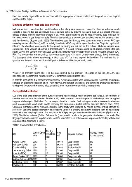
Table 1 Characteristics of study sites
Site
Landfill Open
Year
Site Age
from 2006
(yrs)
Area
(m 2 )
Disposal method
Average tipping
(tonnes per day)
Pattaya (MD1) 2002 4 53,618 Deep landfill 240
Mabtapud (MD2) 2001 5 29,280 Deep landfill 58
Cha-Am (MS1) 2000 6 47,680 Shallow landfill 26
Laemchabang (MD3) 1999 7 71,200 Deep landfill 152
Hua-Hin (MD4) 1996 10 44,160 Deep landfill 46
Samut Prakan (UD1) 1999 7 25,600 Deep dumpsite 80
Nakhon Pathom (UD2) 1997 9 48,781 Deep dumpsite 180
Nonthaburi (UD3) 1982 24 67,367 Deep dumpsite 800
Rayong (US1) 2001 5 35,200 Shallow dumpsite 69
IPCC Expert Meeting Report 56 TFI