ICAS-PAT manual for Design of process monitoring and ... - CAPEC
ICAS-PAT manual for Design of process monitoring and ... - CAPEC
ICAS-PAT manual for Design of process monitoring and ... - CAPEC

Create successful ePaper yourself
Turn your PDF publications into a flip-book with our unique Google optimized e-Paper software.
• Click on the comm<strong>and</strong> button, file name.mot to solve the model. The final value<br />
<strong>of</strong> the variables are shown in Figure 12 (highlighted with red color) <strong>and</strong> the<br />
whole dynamic simulated data is stored in a different file.<br />
• Activate the workbook (maximize the window), <strong>PAT</strong>_Prototype.xls<br />
3.4.3. Click on the comm<strong>and</strong> button, “Load simulation result” .<br />
3.4.4. Click on the comm<strong>and</strong> button, “Select variable”. To analyze the objective<br />
function, select the X axis (independent) variable (usually, ‘Time’ should be<br />
selected as a X axis variable) <strong>and</strong> Y axis variable (objective function) from the<br />
drop-down list <strong>and</strong> select the corresponding symbol <strong>of</strong> the selected variable<br />
(objective function) from the drop-down list.<br />
3.4.5. Click on the comm<strong>and</strong> button, “Operational limits <strong>of</strong> selected variable”.<br />
3.4.6. To plot the selected variable (operational objective), click on the comm<strong>and</strong> button,<br />
“Plot”. If the operational objective is not achieved (if it violates the limits), then<br />
the next step in the procedure needs to be followed.<br />
3.4.7. Select a <strong>process</strong> variable <strong>and</strong> corresponding symbol from the drop-down list<br />
(similarly as mentioned in step 4.4), specify operational limits (similarly as<br />
mentioned in the step 4.5) <strong>and</strong> plot the result (see Figure 11 <strong>for</strong> an example <strong>of</strong> the<br />
result <strong>of</strong> this operation).<br />
3.4.8. Click on the comm<strong>and</strong> button, “Analyze the selected variable”. This comm<strong>and</strong><br />
will open a message box. Select ‘Yes’ if the variable violates the operational limit<br />
<strong>and</strong> ‘No’ if it is within the operational limit.<br />
3.4.9. Repeat steps 4.7 <strong>and</strong> 4.8 <strong>for</strong> each <strong>process</strong> variable involved with the selected<br />
<strong>process</strong> point. The result <strong>of</strong> this step is stored in the result section (see Figure 11,<br />
right).<br />
Open loop simulation data management<br />
• To save the open loop simulation data, write the path <strong>of</strong> the directory where the<br />
data has to be saved <strong>and</strong> click on the comm<strong>and</strong> button, “Save the open loop<br />
simulation data” (see Figure 11).<br />
• To load the saved data click on the comm<strong>and</strong> button, “Load the saved data (open<br />
loop)” (see Figure 11). Follow the steps 4.4 to 4.9 <strong>for</strong> sensitivity analysis based on<br />
the saved data.<br />
14