Remote Health Monitoring for Asset Management

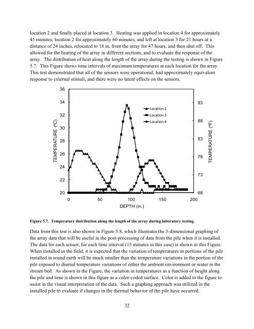
location 2 and finally placed at location 3. Heating was applied in location 4 for approximately
45 minutes, location 2 for approximately 60 minutes, and left at location 3 for 21 hours at a
distance of 24 inches, relocated to 18 in. from the array for 47 hours, and then shut off. This
allowed for the heating of the array in different sections, and to evaluate the response of the
array. The distribution of heat along the length of the array during the testing is shown in Figure
5.7. This Figure shows time intervals of maximum temperatures at each location for the array.
This test demonstrated that all of the sensors were operational, had approximately equivalent
response to external stimuli, and there were no latent effects on the sensors.
36
34
Location 2
93
TEMPERATURE (ºC)
32
30
28
26
Location 3
Location 4
88
83
78
TEMPERATURE (ºF)
24
22
73
20
0 50 100 150 200
DEPTH (in.)
68
Figure 5.7. Temperature distribution along the length of the array during laboratory testing.
Data from this test is also shown in Figure 5.8, which illustrates the 3-dimensional graphing of
the array data that will be useful in the post-processing of data from the pile when it is installed.
The data for each sensor, for each time interval (15 minutes in this case) is shown in this Figure.
When installed in the field, it is expected that the variation of temperatures in portions of the pile
installed in sound earth will be much smaller than the temperature variations in the portion of the
pile exposed to diurnal temperature variations of either the ambient environment or water in the
stream bed. As shown in the Figure, the variation in temperatures as a function of height along
the pile and time is shown in this figure as a color-coded surface. Color is added to the figure to
assist in the visual interpretation of the data. Such a graphing approach was utilized in the
installed pile to evaluate if changes in the thermal behavior of the pile have occurred.
32