Soft-Core Processor Design - CiteSeer

SOFT-CORE PROCESSOR DESIGN
by
Franjo Plavec
A thesis submitted in conformity with the requirements
for the degree of Master of Applied Science
Graduate Department of Electrical and Computer Engineering
University of Toronto
© Copyright by Franjo Plavec 2004

Abstract
Soft-Core Processor Design
Franjo Plavec
Master of Applied Science
Graduate Department of Electrical and Computer Engineering
University of Toronto
2004
Recent advancements in Field Programmable Gate Array (FPGA) technology have
resulted in FPGA devices that support the implementation of a complete computer system
on a single FPGA chip. A soft-core processor is a central component of such a system. A
soft-core processor is a microprocessor defined in software, which can be synthesized in
programmable hardware, such as FPGAs.
The Nios soft-core processor from Altera Corporation is studied and a Verilog
implementation of the Nios soft-core processor has been developed, called UT Nios. The
UT Nios is described, its performance dependence on various architectural parameters is
investigated and then compared to the original implementation from Altera. Experiments
show that the performance of different types of applications varies significantly
depending on the architectural parameters. The performance comparison shows that UT
Nios achieves performance comparable to the original implementation. Finally, the
design methodology, experiences from the design process and issues encountered are
discussed.
ii

Acknowledgments
First, I would like to thank my supervisors Professor Zvonko Vranesic and Professor Stephen
Brown for their advice and support throughout the course of this thesis. I am greatly indebted to
you both. A special thanks to Professor Vranesic for his suggestion of the topic of the thesis and
for all of the hard work with reading the thesis.
I also wish to acknowledge the help of Blair Fort in developing several UT Nios modules and
for developing a game that revealed many bugs in the design, causing endless frustration. Also,
thank you for all the constructive discussions, whether related to the topic of this thesis or not.
Thanks to other people who contributed with their suggestions and ideas. Thanks to Valavan for
pointing me to the Design Space Explorer. Thanks to everyone who attended the Altera research
meetings, soft-processor research meetings, and the FPGA reading group meetings. Thanks to
Nathalie for discovering several bugs and for her interesting questions. Thanks to Lesley for
sharing her experiences with Xilinx tools. Thanks to all the students, staff and the faculty of the
department and the university for making my work and life on campus a pleasant experience.
Special thanks to all the folks in the Croatian Student Association with whom I had many great
times. Also, thanks to Ivan for being a good roommate during the past year.
I thank Professor Sinisa Srbljic for his suggestion to come to Canada and to pursue studies at
U of T. I am greatly indebted to you for your support and advice. I also wish to thank Alex Grbic
and his family. They have come forward and accepted me as a part of their family when I needed
it the most. Special thanks to Tony for driving me home from many late night parties. Also,
thanks to Alex for reading the final draft of this thesis.
I wish to thank my mother for teaching me patience, and my father (may his soul rest in
peace) for teaching me pertinacity. Without you and your continuous support this work would not
have been possible. To my uncle and aunt, Franjo and Vera Plavec for their financial and moral
support during my studies, as well as for encouraging me to take the extra English classes.
Thanks to all of my friends and family for their love and support. Finally, I wish to thank all of
my teachers and professors, past and present. Without you I would not even know how to count,
let alone to design a processor. The patience and effort of many of you have motivated me in
pursuing science.
This work has been financially supported by NSERC, CITR and University of Toronto
Master’s Fellowship. I acknowledge and thank them for their support, for this work would not be
possible without it.
iii

Contents
1 Introduction ................................................................................................................. 1
2 Background.................................................................................................................. 3
2.1. Related work ......................................................................................................... 3
2.2. FPGA technology .................................................................................................. 5
2.3. FPGA Design Flow ............................................................................................... 7
2.4. Stratix FPGA and Quartus II CAD Tool................................................................. 9
3 Altera Nios ..................................................................................................................12
3.1. Nios Architecture .................................................................................................13
3.1.1. Register Structure...................................................................................13
3.1.2. Nios Instruction Set ................................................................................15
3.1.3. Datapath and Memory Organization .......................................................18
3.1.4. Interrupt Handling ..................................................................................19
3.2. Avalon Bus...........................................................................................................22
3.3. Design Flow for a Nios Processor System.............................................................23
3.3.1. SOPC Builder.........................................................................................24
3.3.2. SDK and Software Development Tools...................................................26
4 UT Nios........................................................................................................................28
4.1. UT Nios Datapath.................................................................................................31
4.1.1. Prefetch Unit ..........................................................................................33
4.1.2. Instruction Decoder ................................................................................34
4.1.3. General-Purpose Register File ................................................................36
4.1.4. Operand Handler ....................................................................................38
4.1.5. Branch Unit............................................................................................38
4.1.6. Arithmetic and Logic Unit......................................................................39
4.1.7. Register File Write Multiplexer ..............................................................40
4.1.8. Data Forwarding Logic...........................................................................40
4.1.9. Control Registers....................................................................................42
4.2. Control Unit .........................................................................................................43
5 Performance................................................................................................................47
5.1. Methodology ........................................................................................................47
5.1.1. UT Nios Benchmark Set.........................................................................47
iv

5.1.2. Development Tools ................................................................................50
5.1.3. System Configuration.............................................................................52
5.2. UT Nios Performance...........................................................................................52
5.2.1. Performance Dependence on the Prefetch FIFO Buffer Size ...................53
5.2.2. Performance Dependence on the General-Purpose Register File Size ......56
5.2.3. Performance Dependence on Other Parameters.......................................66
5.3. Altera Nios Performance.......................................................................................67
5.4. Comparison of the UT and Altera Nios .................................................................69
5.4.1. Performance...........................................................................................70
5.4.2. Area Comparison ...................................................................................73
5.4.3. Design Scalability ..................................................................................74
6 Discussion....................................................................................................................76
6.1. Design Process .....................................................................................................76
6.1.1. Development Progress............................................................................76
6.1.2. Design Improvement and Testing ...........................................................78
6.2. Design Analysis....................................................................................................80
6.3. CAD Tools ...........................................................................................................82
7 Conclusions and Future Work ...................................................................................86
7.1. Future Work .........................................................................................................87
8 Bibliography................................................................................................................88
v

List of Figures
Figure 2.1 Simple logic block structure.....................................................................................6
Figure 2.2 FPGA design flow ...................................................................................................8
Figure 3.1 Nios register window structure...............................................................................14
Figure 3.2 Adding custom instructions to Nios [24] ................................................................18
Figure 3.3 Hardware and software design flow for a Nios processor system [44].....................24
Figure 4.1 UT Nios datapath...................................................................................................32
Figure 4.2 Ri8 and Rw instruction formats [23].......................................................................35
Figure 4.3 Data hazard example..............................................................................................41
Figure 4.4 Control unit FSM state diagram .............................................................................44
Figure 5.1 Performance vs. the FIFO buffer size on the ONCHIP system................................53
Figure 5.2 Performance of the test and toy benchmarks vs. the FIFO buffer size on the
SRAM system........................................................................................................54
Figure 5.3 Performance of the application benchmarks vs. the FIFO buffer size on the
SRAM system........................................................................................................55
Figure 5.4 Performance vs. register file size for the ONCHIP system ......................................58
Figure 5.5 Performance vs. register file size for the SRAM system..........................................59
Figure 5.6 Execution tree of the Fibo benchmark ....................................................................61
Figure 5.7 Modelled number of memory accesses vs. the number of the available register
windows for the Fibo benchmark ...........................................................................62
Figure 5.8 Modelled number of memory accesses vs. the number of the available register
windows for simple recursive procedure with recursion depth 8 .............................63
Figure 5.9 Performance comparison of the pipeline optimized for speed and the pipeline
optimized for area on the SRAM system ................................................................69
Figure 5.10 Performance comparison of the toy and test benchmarks on the UT and Altera
Nios based SRAM systems ....................................................................................71
Figure 5.11 Performance comparison of the application benchmarks on the UT and Altera
Nios based SRAM systems ....................................................................................71
Figure 5.12 Performance comparison of the UT and Altera Nios based ONCHIP systems .........73
vi

Chapter 1
Introduction
Since their emergence in the mid-1980s, Field Programmable Gate Arrays (FPGAs) have
become a popular choice for prototyping and production of products in small to moderate
quantities. An FPGA is a special kind of Programmable Logic Device (PLD) that allows
implementation of general digital circuits, limited only by the circuit size. The circuit to be
implemented is defined by programming the device. Over the years, the capabilities of FPGA
devices have grown to the level where a complete multiprocessor system can fit on a single
device [1].
Circuit design for FPGAs is typically done using a CAD (Computer Aided Design) tool.
Modern CAD tools support design entry using several different methods. As the complexity of
the circuits grows, Hardware Description Languages (HDLs) become the only practical choice.
HDLs support circuit description using high-level language constructs. Low-level implementation
details are handled by the CAD tool automatically, so the designer can focus on the design
functionality.
A soft-core processor is a microprocessor fully described in software, usually in an HDL,
which can be synthesized in programmable hardware, such as FPGAs. A soft-core processor
targeting FPGAs is flexible because its parameters can be changed at any time by reprogramming
the device. Traditionally, systems have been built using general-purpose processors implemented
as Application Specific Integrated Circuits (ASIC), placed on printed circuit boards that may have
included FPGAs if flexible user logic was required. Using soft-core processors, such systems can
be integrated on a single FPGA chip, assuming that the soft-core processor provides adequate
performance. Recently, two commercial soft-core processors have become available: Nios [2]
from Altera Corporation, and MicroBlaze [3] from Xilinx Inc.
The main problem with the existing soft-core processor implementations targeting FPGAs is
that they provide very little detail of the implementation and choices made during the
development process. In this thesis, the methodology of soft-core processor development is
investigated. Altera Nios is described in detail, and UT Nios, a soft-core processor
implementation developed as a part of this work is presented. Altera Nios is a 5-stage pipelined
general-purpose Reduced Instruction Set Computer (RISC) soft-core processor, while UT Nios is
a four-stage pipelined processor. Except for some optional components, UT Nios has the
1

functionality equivalent to the Altera Nios and achieves the performance comparable to that of
the Altera Nios. This thesis provides the details of the steps involved in the UT Nios
development, and discusses the design decisions and trade-offs involved. The design cycles in the
FPGA design methodology are much shorter than for ASICs. Therefore, the design decisions
during the UT Nios development process were guided by the feedback from the previous steps.
The thesis shows how this methodology can be used for incremental design improvement.
The UT Nios benchmark set is defined to investigate the performance of the Altera and UT
Nios. The influence of various processor parameters on the performance of both UT and Altera
Nios is investigated, and their performance is compared. The results indicate that the performance
of different applications varies significantly depending on the architectural parameters. Different
applications also achieve different performance when running on the Altera and UT Nios,
although the performance of the two implementations is similar on average. A comparison of the
Altera and UT Nios shows that comparable performance can be achieved by using two different
processor organizations. The thesis discusses the UT Nios design and analyzes the prospects for
design improvements and other future work.
The thesis is organized as follows. Chapter 2 gives an overview of related work, the FPGA
technology and the design flow. In Chapter 3, the Nios architecture is presented, along with the
supporting software tools. Chapter 4 describes the details of the UT Nios architecture.
Experimental results and the methodology used to measure the performance of UT Nios are
presented in Chapter 5. In Chapter 6, a discussion of the design and experimental results is given.
Chapter 7 concludes the thesis and gives an overview of the future work.
2

Chapter 2
Background
Soft-core processors are one aspect of the trend in architecture generally known as
reconfigurable computing. Recent developments in FPGA technology made FPGAs a suitable
target for processor implementations. FPGAs can be reprogrammed, so the processor parameters
can be changed during the lifetime of the product, if the need arises. However, an FPGA
implementation of a soft-core processor will typically provide lower performance than the
corresponding ASIC design. In this chapter we give an overview of the related work, and put soft-
core processors in the context of reconfigurable computing. We also review the FPGA technology
and CAD flow for FPGAs.
2.1. Related work
The concept of reconfigurable computing has been in existence since the early 1960s [4].
Reconfigurable computing systems use some form of programmable hardware to accelerate
algorithm execution. Computation intensive parts of the algorithm are mapped to the
programmable hardware, while the code that cannot be efficiently mapped is usually executed on
a general-purpose processor. Depending on the proximity of programmable hardware to the
general-purpose processor, a system is said to be closely or loosely coupled. In a closely coupled
system, reconfigurable resources allow customization of the processor’s functional units. On the
other end, reconfigurable hardware in a loosely coupled system can be a standalone network unit.
Reconfigurable systems are usually categorized between these two extremes. There has been a lot
of research in the area of reconfigurable computing. An extensive survey of reconfigurable
systems can be found in [4].
In reconfigurable systems, performance critical parts of the application are implemented in
hardware. Since various systems tend to use common algorithms, many of the developed
components can be reused. Reusable components come in the form of intellectual property (IP)
cores. An IP core is a standard block of logic or data that can be used to build a larger or more
complex system. IP cores are divided into three categories, depending on the level of
optimization, and flexibility of reuse: soft cores, firm cores, and hard cores [5]. A soft core is
usually a synthesizable HDL specification that can be retargeted to various semiconductor
3

processes. A firm core is generally specified as a gate-level netlist, suitable for placement and
routing, while a hard core also includes technology-dependent information like layout and timing.
Generally, soft cores provide the highest flexibility, allowing many core parameters to be
changed prior to synthesis, while hard cores provide little or no flexibility. Some cores are
patented and copyrighted, while others are freely available under the GNU Public License (GPL)
[6].
Recent developments in FPGA technology, like the addition of substantial amounts of
memory, have made FPGAs suitable for soft-core processor implementation. In the past few
years, two popular soft-core processors have emerged: Nios [2] from Altera Corporation, and
MicroBlaze [3] from Xilinx Inc. Both Altera and Xilinx also offer FPGAs containing hard cores.
Altera’s Excalibur devices [7] include the ARM922T core, while Xilinx integrates the PowerPC
core in their PowerPC Embedded Processor Solution [8].
Since UT Nios, developed as a part of this thesis, is a soft-core processor, the rest of the thesis
will focus on soft-cores and related issues. The Nios architecture and the Altera Nios soft-core
processor are described in more detail in the next chapter. MicroBlaze is a 32-bit general-purpose
RISC microprocessor optimized for implementation in Xilinx FPGAs [9]. The MicroBlaze
architecture is fully orthogonal, and contains 32 32-bit registers. An instruction word is 32-bits
wide, and supports up to 3 operands, and 2 addressing modes. Instructions are executed in a
single-issue 3-stage pipeline. Since modern Xilinx FPGAs contain considerable amounts of
memory, on-chip memory can be used to store data and instructions. Off-chip memory can also
be used, with optional data and instruction cache memories. Data and instruction caches are
separate, and their size is configurable. Depending on the configuration and target device,
MicroBlaze can run at the clock speed from 65 to 150 MHz, achieving performance between 43
and 125 Dhrystone MIPS [3]. Xilinx also offers a PicoBlaze, an 8-bit microcontroller targeting
applications requiring complex, but not time-critical state machines [10].
In addition to the MicroBlaze processor, Xilinx also provides many other soft cores needed to
build a complete microprocessor system. Cores include memory controllers, interrupt controllers,
Ethernet controllers, UARTs (UART - Universal Asynchronous Receiver/Transmitter), timers,
buses, and others. Using these cores and on-chip memory, all components of a computer system
can be placed on a single FPGA. This concept is known as a system on a programmable chip
(SOPC). Aside from the commercial soft-core processors, several soft-core processors and other
cores are available under the GPL license [6].
A common characteristic of many soft-core processor projects is that they provide very little
detail on the methodology used in a processor design. An impression is that the processors were
4

uilt using techniques proven to be appropriate for ASIC processors. However, having in mind
the differences in the implementation technologies, it is not obvious if the same rules that hold for
ASIC designs can be applied to designs for FPGAs. This work differs from previous work in that
it tries to give an insight into the development process, including the design choices and trade-
offs in developing a soft-core processor. Since the design cycles in the FPGA design
methodology are much shorter than for ASICs, it is practical to improve the design incrementally,
using feedback from the previous steps. Many decisions in this work were guided by such
feedback, not by the traditional wisdom. The result is an architecture, significantly different than
the Altera Nios, with an average performance very close to the original processor. Although the
FPGA design flow reduces the time needed to explore the design space, the design space is still
vast, so this work can serve as a basis for future research.
2.2. FPGA technology
FPGA devices are programmable to implement arbitrary user logic. To support this
programmability, FPGA devices contain three types of resources: logic blocks, I/O blocks, and
programmable interconnection.
Most FPGAs contain logic blocks that consist of a lookup table (LUT), and a flip-flop. A LUT
can be programmed to implement any logic function of its inputs. A LUT with n inputs is called
an n-LUT. An n-LUT is internally implemented as a set of 2-to-1 multiplexers, functioning as a
2 n -to-1 multiplexer. Multiplexer inputs are programmable, while select lines are used for inputs of
the implemented function. Research has shown that 4-LUTs are an optimal choice for
FPGAs [11].
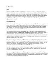
Figure 2.1 shows an example of a logic block consisting of a 3-LUT, and a flip-flop. An 8-to-
1 multiplexer in a LUT is implemented using 2-to-1 multiplexers. Therefore, the propagation
delay from inputs to the output is not the same for all the inputs. Input IN 1 experiences the
shortest propagation delay, because the signal passes through fewer multiplexers than signals IN
2 and IN 3. Since a LUT can implement any function of its input variables, inputs to the LUTs
should be mapped in such a way that the signals on a critical path pass through as few
multiplexers as possible. Logic blocks also include a flip-flop to allow the implementation of
sequential logic. An additional multiplexer is used to select between the LUT and the flip-flop
output. Logic blocks in modern FPGAs [12] are usually more complex than the one presented
here.
5

� ��¥
� ���
� ���
¢¤£¦¥
¢¤£¦¥
¢¤£¦¥
¢¤£¦¥
¢¤£¦¥
¢¤£¦¥
¢¤£¦¥
¢¤£¦¥
Each logic block can implement only small functions of several variables. Programmable
interconnection, also called routing, is used to connect logic blocks into larger circuits performing
the required functionality. Routing consists of wires that span one or more logic blocks.
Connections between logic blocks and routing, I/O blocks and routing, and among wires
themselves is programmable, which allows for the flexibility of circuit implementation. Routing
is a very important aspect of FPGA devices, because it dominates the chip area and most of the
circuit delay is due to the routing delays [11].
�����
I/O blocks in an FPGA connect the internal logic to the outside pins. Depending on an actual
device, most pins can be configured as either input, output, or bidirectional. Devices supporting
more than one I/O standard allow configuration of different pins for different standards [12].
Programmability of FPGAs is commonly achieved using one of three technologies: SRAM
cells, antifuses, and floating gate devices. Most devices use SRAM cells. The SRAM cells drive
pass transistors, multiplexers, and tri-state buffers, which in turn control the configurable routing,
6
�����
Figure 2.1 Simple logic block structure
¡
�����������
§©¨��

logic and I/O blocks [11]. Since the content of SRAM cells is lost when the device is not
powered, the configuration needs to be reloaded into the device on each power-up. This is done
using a configuration device that loads the configuration stored in some form of non-volatile
memory.
Programmability of FPGAs comes at a price. Resources necessary for the programmability
take up chip area and consume power. Therefore, circuits implemented in FPGAs take up more
area and consume more power than in equivalent ASIC implementations. Furthermore, since the
routing in FPGAs is achieved using programmable switches, as opposed to metal wires in ASICs,
circuit delays in FPGAs are higher. Because of that, care has to be taken to exploit the resources
in an FPGA efficiently. Circuit speed is important for high-throughput applications like Digital
Signal Processing (DSP), while power is important for embedded applications. CAD tools are
used by the designer to meet these requirements.
2.3. FPGA Design Flow
Designing a complex system targeting FPGAs would be virtually impossible without CAD
tools. The CAD tools convert the user’s specification into an FPGA configuration that
implements the specified functionality, while optimizing one or more design parameters.
Common optimizations include reducing the chip area, increasing the speed, and reducing the
power usage. The CAD tools perform a set of steps to map the design specification to an FPGA.
Figure 2.2 shows the design flow of typical CAD tools targeting FPGAs [11].
Input to a CAD tool is a high-level circuit description, which is typically provided using a
hardware description language (HDL). VHDL (Very High Speed Integrated Circuit Hardware
Description Language) and Verilog HDL are the two most popular HDLs in use today. An HDL
circuit description is converted into a netlist of basic gates in the synthesis step of the design flow.
The netlist is optimized using technology-independent logic minimization algorithms. The
optimized netlist is mapped to the target device using a technology-mapping algorithm.
A minimization algorithm ensures that the circuit uses as few logic blocks as possible. Further
optimizations that exploit the structure of the underlying FPGA are also performed. For instance,
some FPGAs group logic blocks in clusters, with high connectivity among the blocks inside the
cluster, and less routing resources connecting logic blocks in different clusters. This is usually
referred to as hierarchical routing. The synthesis tool will use information on the cluster size and
connectivity to map logic that requires many connections inside a cluster. This optimization is
7

Figure 2.2 FPGA design flow
commonly known as clustering [11]. The final result of synthesis is a netlist of logic blocks, a set
of LUT programming bits, and possibly the clustering information.
The placement algorithm maps logic blocks from the netlist to physical locations on an FPGA.
If the clustering was performed during the synthesis step, clustered LUTs are mapped to physical
clusters. Logic block placement directly influences the amount of routing resources required to
implement the circuit. A placement configuration that requires more routing resources than is
available in the corresponding portion of the device cannot be routed. Hence, the circuit cannot be
implemented in an FPGA with that placement configuration, and a better placement must be
found, if one exists. Since the number of possible placements is large, metaheuristic algorithms
[13] are used. The most commonly used algorithm is simulated annealing. “Simulated annealing
mimics the annealing process used to gradually cool molten metal to produce high-quality metal
objects” [11]. The algorithm starts with a random placement and incrementally tries to improve it.
The quality of a particular placement is determined by the routing required to realize all the
connections specified in the netlist. Since the routing problem is known to be NP-complete [14], a
cost function approximating the routing area is used to estimate the quality of the placement. If
the cost function is associated with routing resources only, the placement is said to be routability-
or wire-length-driven. If the cost function also takes into account circuit speed, the placement is
8

timing-driven [11]. Although simulated annealing produces suboptimal results, a good choice of
the cost function yields average results that are reasonably close to optimal.
Once the placement has been done, the routing algorithm determines how to interconnect the
logic blocks using the available routing. The routing algorithm can also be timing- or
routability-driven. While a routability-driven algorithm only tries to allocate routing resources so
that all signals can be routed, a timing-driven algorithm tries also to minimize the routing delays
[15]. The routing algorithm produces a set of programming bits determining the state of all the
interconnection switches inside an FPGA.
The final output the CAD tools produce is the FPGA programming file, which is a bit stream
determining the state of every programmable element inside an FPGA. Design flow, including
synthesis, placement and routing is sometimes referred to as the design compilation. Although the
term synthesis is also commonly used, we will use the term design compilation to avoid
confusion between the synthesis step of the design flow, and the complete design flow.
Although design compilation does not generally require the designer’s assistance, modern
tools allow the designer to direct the synthesis process by specifying various parameters. Even
variations in the initial specification can influence the quality of the final result (examples of such
behaviour will be shown later in the thesis). This suggests that the designer should understand the
CAD tools and the underlying technology to fully exploit the capabilities of both tools and the
device. In the following section we give an overview of the CAD tool and the FPGA device used
in the thesis.
2.4. Stratix FPGA and Quartus II CAD Tool
The previous two sections presented a general FPGA architecture and CAD design flow. In
this section, the Stratix FPGA device family [12] used for the implementation of UT Nios is
presented. The CAD tool Quartus II [16], used for the synthesis of the UT Nios design, is also
described.
The terminology used in Stratix documentation [12] is somewhat different than that presented
in section 2.1. A logic element (LE) is very similar to the logic block depicted in Figure 2.1. It
consists of a 4-LUT, a register (flip-flop), a multiplexer to choose between the LUT and the
register output, and additional logic required for advanced routing employed in Stratix. Special
kinds of interconnection; LUT chains, register chains, and carry chains, are used to minimize the
routing delay and increase capabilities of groups of LEs. Groups of 10 LEs are packed inside
clusters called Logic Array Blocks (LABs), with a hierarchical routing structure [12].
9

The Stratix FPGA device family has a much more complex structure than the general FPGA
described in section 2.1. In addition to logic blocks, routing, and I/O blocks, Stratix devices also
contain DSP blocks, phase-locked loops (PLLs), and memory blocks. As already mentioned,
memory is the key component that makes an FPGA suitable for SOPC designs. Devices in the
Stratix family contain anywhere from 920,448 to 7,427,520 memory bits. Several different types
of memory blocks are available, each one suited to a particular application. Memory blocks
support several modes of operation, including simple dual-port, true dual-port, and single-port
RAM, ROM, and FIFO buffers. Some memory block types can be initialized at the time the
device is configured [12]. In this case the memory initialization bits are a part of the FPGA
programming file.
All the memory available in Stratix devices is synchronous. All inputs to a memory block are
registered, so the address and data are always captured on a clock edge. Outputs can be registered
for pipelined designs. Synchronous memory offers several advantages over asynchronous
memory. Synchronous memory generates a write strobe signal internally, so there is no need for
external circuitry. Performance of the synchronous memory is the same or better than
asynchronous memory, providing that the design is pipelined [17].
Quartus II provides a set of tools for circuit designs targeting Altera programmable devices.
These tools include design editors, compilation and simulation tools, and device programming
software. Design specification can be entered using one or more of the following formats:
schematic entry, VHDL, Verilog HDL, Altera HDL (AHDL), EDIF netlist, and Verilog Quartus
Mapping File (VQM) netlist. AHDL is an Altera specific HDL integrated into Quartus II. EDIF
and VQM are two netlist specification formats [18]. Netlist input formats are useful when a third
party synthesis tool is used in the design flow. Output of the third party tool can be fed to
Quartus, which performs placement and routing (also called fitting in Quartus terminology) for
Altera FPGAs. This is especially useful for legacy designs that include language constructs or
library components specific to other synthesis tools. Various parameters guiding the compilation
process can be set, and the process can be automated using scripting.
Quartus II includes a library of parameterizable megafunctions (LPM), which implement
standard building blocks used in digital circuit design. Library megafunctions may be
parameterized at design time to better suite the needs of a system being designed. Using the
megafunctions instead of implementing the custom blocks reduces the design time. The
megafunctions may be implemented more efficiently in the target FPGA than the custom design,
although that is not necessarily always the case [16]. There are two ways a megafunction can be
included in HDL design. It may be explicitly instantiated as a module, or it can be inferred from
10

the HDL coding style. To ensure that the desired megafunction will be inferred from the HDL,
the coding style guidelines outlined in [16] should be followed.
Aside from the design flow steps described in the section 2.3, the Quartus II design flow
includes two optional steps: timing analysis and simulation. Timing analysis provides information
about critical paths in a design by analyzing the netlist produced by the fitter. Simulation is used
for design verification by comparing the expected output with the output of the design simulation.
The Quartus II simulator supports two modes of simulation; functional and timing. Functional
simulation verifies the functionality of the netlist produced by synthesis. At that level, timing
parameters are unknown, since there is no information on mapping into the physical device.
Therefore, the functional simulation ignores any timing parameters and assumes that the
propagation delays are negligible. The timing simulation extracts the timing information from the
fitting results, and uses it to simulate the design functionality, including timing relations among
signals. The timing simulation gives more precise information about the system behaviour at the
expense of increased simulation time.
Quartus II also supports the use of other Electronic Design Automation (EDA) tools. One such
tool is ModelSim [19], the simulation tool which was particularly useful for the work in this
thesis. In addition to functional and timing simulation, ModelSim also supports behavioural
simulation. The behavioural simulation verifies the functionality of the circuit description,
without any insight into actual implementation details. For instance, if the circuit specification is
given in an HDL, the behavioural simulator would simulate the HDL code line by line; like a
program in a high-level language. Unlike the functional simulator, the behavioural simulator does
not take into account how the circuit specification maps into logic gates, or if it can be mapped at
all. A design that passes the behavioural verification may not function correctly when
implemented in logic, since it is unknown how it maps to the hardware.
To make sure that the behavioural description will compile and produce a circuit with
intended behaviour, designers should follow the design recommendations provided in the Quartus
II documentation [16]. This is especially true when writing HDL code. Both Verilog and VHDL
were designed as simulation languages; only a subset of the language constructs is supported for
synthesis [20,21]. Therefore, not all syntactically correct HDL code will compile into the
functionality corresponding to the results of the behavioural simulation.
In this chapter, an overview of the previous work in the area of reconfigurable computing has
been presented. Design methodology, and hardware and software tools used in this thesis have
also been presented. The next chapter presents the Altera Nios soft-core processor and supporting
tools in more detail.
11

Chapter 3
Altera Nios
Altera Nios [2] is a general-purpose RISC soft-core processor optimized for implementation in
programmable logic chips. Throughout this thesis we use the term Nios for the instruction set
architecture described in [22] and [23]. The term Altera Nios is used for the Nios implementation
provided by Altera. The term UT Nios designates the Nios implementation developed as a part of
this work.
Altera Nios is a highly customizable soft-core processor. Many processor parameters can be
selected at design time, including the datapath width and register file size. The instruction set is
customizable through selection of optional instructions and support for up to 5 custom
instructions [24]. Instructions and data can be placed in both on- and off-chip memory. For
off-chip memory, there are optional on-chip instruction and data caches. Aside from the processor
and memory, customizable standard peripherals, like UARTs and timers, are also available.
System components are interconnected using an Avalon bus, which is a parameterizable bus
interface designed for interconnection of on- and off-chip processors and peripherals into a
system on a programmable chip [25].
Altera Nios processor has been widely used in industry and academia. In academia it has been
used in networking applications [26], parallel applications [1], and for teaching purposes
[27,28,29]. Information on the use of Nios in industry is not readily available. A partial list of
companies that have used Altera Nios can be found in [30]. Altera Nios is shipped with a standard
set of development tools for building systems. Third party tools and system software are also
available, including a real-time operating system [31].
In this chapter we describe the architectural features of the Altera Nios processor. We also
give an overview of design tools for building Nios systems, and tools for developing system
software. The chapter focuses on the architectural features and supporting tools that are directly
relevant to the work presented in this thesis. Details of the architecture and tools can be found in
the referenced literature.
12

3.1. Nios Architecture
The Nios instruction set architecture is highly customizable. At design time, a subset of
available features is selected. For instance, the designer can select a 16- or 32-bit datapath width
[22,23]. Throughout the thesis, the term 16-bit Nios is used for Nios with the 16-bit datapath,
while 32-bit Nios refers to Nios with the 32-bit datapath. In the context of both 16- and 32-bit
Nios, the term word is used for 32 bits, halfword for 16 bits, and byte for 8 bits. Most instructions
are common to both 16- and 32-bit Nios processors. In this section we present both instruction
sets, noting the instructions which are datapath-width specific.
3.1.1. Register Structure
The Nios architecture has a large, windowed general-purpose register file, a set of control
registers, a program counter (PC), and a K register used as a temporary storage for immediate
operands. All registers, except the K register, are 16-bits wide for 16-bit Nios, and 32-bits wide
for 32-bit Nios. The K register is 11 bits wide for both processors.
The total size of the general-purpose register file is configurable. However, only a window of
32 registers can be used at any given time. The Nios register window structure is similar to the
structure used in the SPARC microprocessor [32]. A register window is divided into four groups
of 8 registers: Global, Output, Local, and Input registers. The current window pointer (CWP)
field in the STATUS control register determines which register window is currently in use. The
structure of the register windows is depicted in Figure 3.1.
Changing the value of the CWP field changes the set of registers that are visible to the
software executing on the processor. This is typically done using SAVE and RESTORE
instructions. The SAVE instruction decrements the CWP, opening a new set of Local and Output
registers. It is usually issued on entry to a procedure. The RESTORE instruction increments the
CWP, and is usually issued on exit from the procedure. Input registers overlap with the calling
procedure’s Output registers, providing an efficient way for argument passing between
procedures. Global registers are shared by all register windows. This means that the same set of
Global registers is available in all windows and thus suitable for keeping global variables. The
number of available register windows depends on the total size of the register file. Altera Nios
can be configured to use 128, 256, or 512 registers, which provides 7, 15, and 31 register
windows, respectively. One register window is usually reserved for fast interrupt handling if the
interrupts are enabled.
13

�¦��¥���¥
� �§¥�¨��
��§©�¦£ �
§ ¨��©¥�¨��
� ���
�����
� � ¢
����¢
�����
����¢
General-purpose registers are accessible in the assembly language using several different
names. Global registers are accessible as %g0 to %g7, or %r0 to %r7. Output registers are known
as %o0 to %o7, or %r8 to %r15, with %o6 also being known as %sp (stack pointer). Local
registers can be accessed as %L0 to %L7, or %r16 to %r23. Input registers are accessible as %i0
to %i7, or %r24 to %r31, with %i6 also being used as %fp (frame pointer).
�¦��¥
� �§¥�¨��
��§©�¨£©�
§ ¨��¦¥�¨��
��§¢¡¤£©�
In addition to the general-purpose registers, Nios also has 10 control registers: %ctl0 through
%ctl9. The STATUS control register (%ctl0) keeps track of the status of the processor, including
the state of the condition code flags, CWP, current interrupt priority (IPRI), and the interrupt
enable bit (IE). The 32-bit Altera Nios STATUS register also includes the data cache enable (DC)
and instruction cache enable (IC) bits. On a system reset, the CWP field is set to the highest valid
value. This value is stored in HI_LIMIT field of the WVALID register (%ctl2), which stores the
highest and the lowest valid CWP value. Crossing either of these limits causes an exception,
providing the exception support was enabled at design time and exceptions are enabled (IE bit is
set). The control register ISTATUS (%ctl1) is used for fast saving of the STATUS register when
the exception occurs. Control registers CLR_IE (%ctl8) and SET_IE (%ctl9) are virtual registers.
A write operation to these registers is used to set and clear the IE bit in the STATUS register. The
14
��� �
��� ¢
�¦��¥���¥
� �§¥�¨��
��§ �¦£©�
§ ¨��¦¥�¨��
Figure 3.1 Nios register window structure

esult of a read operation from these registers is undefined. Other control registers include CPU
ID (%ctl6) which identifies the version of the Altera Nios processor, and several reserved
registers whose function is not defined in the documentation [22,23]. The 32-bit Altera Nios also
has control registers ICACHE (%ctl5) and DCACHE (%ctl7), used to invalidate cache lines in
the instruction and data caches, respectively. Both ICACHE and DCACHE are write-only
registers. Reading these registers produces an undefined value.
Control registers can be directly read and written to by using instructions RDCTL and
WRCTL, respectively. Control registers can also be modified implicitly as a result of other
operations. Condition code flags are updated by arithmetic and logic instructions depending on
the result of their operation. Fields IPRI and IE bit in the STATUS register are modified, and the
old value of the STATUS is stored to the ISTATUS register when the interrupt occurs.
The register set also includes the program counter (PC) and the K register. The program
counter holds the address of the instruction that is being executed. K is an 11-bit register used to
form longer immediate operands. Since both 16- and 32-bit Nios have an instruction word that is
16-bits wide, it is not possible to fit a 16-bit immediate operand into the instruction word. The
16-bit immediate value is formed by concatenating the 11-bit value in the K register with the 5-bit
immediate operand from the instruction word. The K register is set to 0 by any instruction other
than PFX, which is used to load the K register with the 11-bit immediate value specified in the
instruction word. The PFX instruction and the instruction following it are executed atomically.
Interrupts are disabled until the instruction following the PFX commits. The PFXIO instruction is
available only in the 32-bit Altera Nios; it behaves just like the PFX instruction except that it
forces the subsequent memory load operation to bypass the data cache.
3.1.2. Nios Instruction Set
The Nios instruction set is optimized for embedded applications [33]. To reduce the code size,
all instruction words are 16-bits wide in both 16- and 32-bit Nios architectures. Previous research
on other architectures has shown that using the 16-bit instruction width can produce up to 40%
reduction in code size compared to the 32-bits wide instruction word [34]. Nios is a load-store
architecture with the two-operand instruction format and 32 addressable general-purpose
registers. More than ten different instruction formats exist to accommodate the addressing modes
available.
The Nios instruction set supports several addressing modes, including 5/16-bit immediate,
register, register indirect, register indirect with offset, and relative mode. Many arithmetic and
logic instructions use 5-bit immediate operands specified in the instruction word. If such an
15

instruction is immediately preceded by the PFX instruction, the K register is used to form a 16-bit
immediate operand. Otherwise, a 5-bit immediate operand is used. This is referred to as the
5/16-bit immediate addressing mode. The K register value is also used as the only immediate
operand by some instructions. Other instructions use immediate operands of various lengths
specified as a part of the instruction word. Logic instructions AND, ANDN, OR and XOR use
either register or 16-bit immediate addressing mode, depending on whether the instruction is
preceded by the PFX instruction or not. If the instruction is preceded by the PFX instruction, the
5-bit immediate value is used to form a 16-bit immediate operand. Otherwise, the same 5 bits are
used as a register address. Register indirect and register indirect with offset addressing modes are
used for memory accesses. All load instructions read a word (or halfword for 16-bit Nios) from
memory. Special store instructions allow writing a partial word into memory. Relative addressing
mode is used by branch instructions for target address calculation.
In addition to the addressing modes already mentioned, some instructions also use implicit
operands, like %fp and %sp. The term stack addressing mode is sometimes used for instructions
that use %sp as an implicit operand. Similarly, the term pointer addressing mode is used for
instructions that use one of the registers %L0 to %L3 as a base register. The pointer addressing
mode requires fewer bits in the instruction word for register addressing, since only 4 registers can
be used. In the stack addressing mode, the implicit operand (%sp) is encoded in the OP code.
Control-flow instructions include unconditional branches, jumps, and trap instructions; and
conditional skip instructions. Branches and jumps have delay slot behaviour. The instruction
immediately following a branch or a jump is said to be in the delay slot, and is executed before
the target instruction of the branch. The PFX instruction and the control-flow instructions are not
allowed in the delay slot of another control-flow instruction.
Instructions BR and BSR are unconditional branch instructions. The target address is
calculated relative to the current PC. An 11-bit immediate operand is used as the offset. The
offset is given as a signed number of halfwords, and is therefore limited to the memory window
of 4 KB. The BSR instruction is similar to the BR instruction, but it also saves the return address
in register %o7. The return address is the address of the second instruction after the branch,
because the instruction in the delay slot is executed prior to branching. Jump instructions JMP
and CALL are similar to BR and BSR, respectively, except that the target address is specified in a
general-purpose register. Instructions TRAP and TRET are used for trap and interrupt handling,
and do not have the delay slot behaviour.
Conditional execution in the Nios architecture is done by using one of five conditional skip
instructions. A conditional skip instruction tests the specified condition, and if the condition is
16

satisfied the instruction that follows is skipped (i.e. not executed). The instruction following the
skip instruction is fetched regardless of the result of the condition test, but it is not committed if
the skip condition is satisfied. If this instruction is PFX, then both the PFX instruction and the
instruction following it are skipped to insure the atomicity of the PFX and the subsequent
instruction. Conditional jumps and branches are implemented by preceding the jump or branch
instruction with a skip instruction. The concept of conditional skip instructions is not new to the
Nios architecture. It was used previously in the PDP-8 architecture [35], and is still used in some
modern microcontrollers [36]. The conditional skip instructions use a concept similar to
predicated execution, which can be useful in eliminating short conditional branches [34].
Altera Nios documentation states that “Nios uses a branch-not-taken prediction scheme to
issue speculative addresses” [37]. This is only a simplified view of the real branch behaviour. All
branches and jumps in Nios architecture are in fact unconditional. Conditional branching is
achieved by using a combination of a branch and one of the skip instructions. Skip instructions
are conditional, and since the instruction immediately following a skip is fetched regardless of the
skip outcome, the prediction scheme could be called skip-not-taken. Hence, if the instruction
immediately following the skip is a branch, it will always be fetched. Depending on the pipeline
implementation, other instructions following the branch will be fetched before the outcome of the
skip instruction is known. Therefore, instructions after the branch are fetched before it is actually
known whether the branch will execute or not, which justifies the use of the name branch-not-
taken for this prediction scheme. It is worth noting that the only support in the hardware,
necessary to implement the branch-not-taken prediction scheme, is flushing of the pipeline in a
case when the branch is actually taken.
The Nios instruction set supports only a basic set of logic and arithmetic instructions. Logic
instructions include the operations AND, OR, NOT, XOR, logical shifts, bit generate, and others.
Optionally, rotate through carry (for 1 bit only) can be included in the instruction set. Arithmetic
instructions include variants of addition, subtraction, 2’s-complement arithmetic shift, and
absolute value calculation. Multiplication operation can optionally be supported in hardware by
using one of two instructions: MSTEP or MUL. The MSTEP instruction performs one step of the
unsigned integer multiplication of two 16-bit numbers. The MUL instruction performs an integer
multiplication of two signed or unsigned 16-bit numbers. If neither MSTEP nor MUL are
implemented, software routines will be used for multiplication. Hardware implementation is
faster, but consumes logic resources in the FPGA. The MSTEP and MUL instructions are only
supported for 32-bit Nios.
17

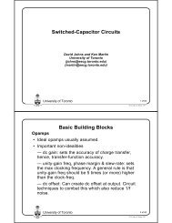
In addition to optional instructions, the Altera Nios instruction set can be customized by
defining up to five user-defined (custom) instructions. Instruction encoding reserves five OP
codes for user instructions. In the assembly language, user instructions can be referred to using
mnemonics USR0 through USR4. User instruction functionality is defined as a module with a
predefined interface [24]. Functionality specification can be given using any of the design entry
formats supported by Quartus II. Both single-cycle (combinational), and multi-cycle (sequential)
operations are allowed in user instructions. The number of cycles it takes for a multi-cycle
operation to produce the result has to be fixed and declared at the system design time. Custom
instruction logic is added in parallel to the functional units of the Nios processor, which
corresponds to a closely coupled reconfigurable system. A module with user instruction
specification can also interface user logic external to the processor, as shown in Figure 3.2 [24].
3.1.3. Datapath and Memory Organization
The Altera Nios datapath is organized as a 5-stage single-issue pipeline with separate data and
instruction masters. The data master performs memory load and store operations, while the
instruction master fetches the instructions from the instruction memory. Many pipeline details are
not provided in the Altera literature.
Figure 3.2 Adding custom instructions to Nios [24]
18

Most instructions take 5 cycles to execute. Execution time of the MUL instruction varies from
5 to 8 cycles, depending on the FPGA device it is implemented in. MSTEP and shift instructions
take 6 cycles to execute. Memory operations take 5 or more cycles to execute, depending on the
memory latency and bus arbitration. Although each instruction takes at least 5 cycles to execute,
due to pipelined execution, one instruction per cycle will finish its execution in the ideal case. In
reality, less than one instruction will commit per cycle, since some instructions take more than 5
cycles to execute. The pipeline implementation is not visible to user programs, except for the
instructions in the delay slot, and the WRCTL instruction. An instruction in the delay slot
executes out of the original program order. Any WRCTL instruction modifying the STATUS
register has to be followed by a NOP instruction. NOP is a pseudo instruction implemented as
MOV %r0, %r0.
Systems using the Nios processor can use both on- and off-chip memory for instruction and
data storage. Memory is byte addressable, and words and halfwords are stored in memory using
little-endian byte ordering. All memory addresses are word aligned for 32-bit Nios, and halfword
aligned for 16-bit Nios. Special control signals, called byte-enable lines, are used when a partial
word has to be written to the memory. Systems using off-chip memory can use the on-chip
memory as instruction and data caches. Caches are direct-mapped with write-through write
policy for the data cache. The instruction cache is read-only. If a program writes to the instruction
memory, the corresponding lines in the instruction cache have to be invalidated. Cache support is
only provided for the 32-bit Altera Nios.
Several Nios datapath parameters can be customized. The pipeline can be optimized for speed
or area. The instruction decoder can be implemented in logic or in memory. Implementation in
logic is faster, while memory implementation uses on-chip memory and leaves more resources for
user-logic. According to [38], both 16- and 32-bit Nios can run at clock speeds over 125 MHz.
This number varies depending on the target FPGA device.
3.1.4. Interrupt Handling
There are three possible sources of interrupts in the Nios architecture: internal exceptions,
software interrupts, and I/O interrupts. Internal exceptions occur because of unexpected results in
instruction execution. Software-interrupts are explicit calls to trap routines using TRAP
instruction, often used for operating system calls. I/O interrupts come from I/O devices external
to the Nios processor, which may reside both on and off-chip.
The Nios architecture supports up to 64 vectored interrupts. Internal exceptions have
predefined exception numbers, while software-interrupts provide the exception number as an
19

immediate operand. The interrupt number for an I/O interrupt is provided through a 6-bit input
signal. In most systems, the automatically generated Avalon bus provides this functionality, so
the I/O devices need to provide only a single output for an interrupt request. Interrupt priorities
are defined by exception numbers: the lowest exception number has the highest priority.
Internal exceptions can only occur as a result of executing SAVE and RESTORE instructions.
If the SAVE instruction is executed while the lowest valid register window is in use
(CWP = LO_LIMIT), a register window underflow exception occurs. Register window overflow
exception, on the other hand, happens when the highest valid register window is in use
(CWP = HI_LIMIT), and the RESTORE instruction is executed. Register window underflow and
overflow exceptions have exception numbers 1 and 2, respectively. These exceptions ensure that
the data in the register window is not overwritten due to the underflow or overflow of the CWP
value. Register window underflow/overflow exceptions can be handled in two ways: the user
application can terminate with an error message, or the code that virtualizes the register file
(CWP Manager) can be executed. The CWP Manager stores the contents of the register file to
memory on the window underflow, and restores the values from the memory on the window
overflow exception. The CWP Manager is included in the Nios Software Development Kit (SDK)
library by default. Only SAVE and RESTORE instructions can cause register window
underflow/overflow exceptions. Modifying the CWP field using the WRCTL instruction cannot
cause exceptions.
All interrupts, except the interrupt number 0 and software interrupts, are handled equivalently.
First of all, an interrupt is only processed if interrupts are enabled (IE bit in the status register is
set), and the interrupt priority is higher than the current interrupt priority (interrupt number is less
than the IPRI field in the status register). Interrupt processing is performed in several steps. First,
the STATUS control register is copied into the ISTATUS register. Next, the IE bit in the
STATUS register is set to 0, CWP is decremented (opening a new register window), and the IPRI
field is set to the interrupt number of the interrupt being processed. At the same time, the return
address is stored in general-purpose register %o7. The return address is the address of the
instruction that would have executed if the interrupt had not occurred. Finally, the address of the
interrupt handling routine is fetched from the corresponding entry in the vector table, and the
control is transferred to that address. Interrupt handling routines can use registers in the newly
opened window, which reduces the interrupt handling latency because the handler routine does
not need to save any registers. The only interrupt that does not open a new window is the register
window overflow exception. The CWP value remains at HI_LIMIT when the register window
overflow exception occurs. This is acceptable, because the program will either terminate or the
20

contents of the register window will be restored from the memory. Interrupt handler routines use
the TRET instruction with register %o7 as an argument to return the control to the interrupted
program. Before returning control, the TRET instruction also restores the STATUS register from
the ISTATUS register. If the IE bit was set prior to the occurrence of the interrupt, then restoring
the STATUS register effectively re-enables interrupts, since the STATUS register was saved
before the interrupts were disabled.
Software interrupts are processed regardless of the values of IE and IPRI fields in the status
register. The return address for the software interrupt is the address of the instruction immediately
following the TRAP, since the TRAP instruction does not have the delay slot behaviour. Software
interrupts are in other respects handled as described above. Interrupt number 0 is a non-maskable
interrupt, and its behaviour is not dependent on IE or IPRI fields. It does not use the vector table
entry to determine the interrupt handler address. It is used by the Nios on-chip instrumentation
(OCI) debug module, which is an IP core designed by First Silicon Solutions (FS2) Inc [39]. The
OCI debug module enables advanced debugging by connecting directly to the signals internal to
the Altera Nios CPU [23].
Exceptions do not occur if an unused OP code is issued. An unused OP code is treated as a
NOP by the Altera Nios [40]. Issuing the MUL instruction on a 32-bit Altera Nios that does not
implement the MUL instruction in hardware does not cause an exception, and the result is
undefined [37]. Similarly, the result of the PFXIO operation immediately before any instruction
other than LD or LDP is undefined [23]. Available documentation does not specify the effect of
issuing other optional instructions (e.g. RLC and RRC) when there is no appropriate support in
hardware.
Interrupts are not accepted when the instruction in the branch delay slot is executed because
that would require saving two return addresses: the branch target address and the delay slot
address. Although this behaviour is not specified in the documentation, it follows directly from
[41]. To save logic resources on the FPGA chip, interrupt handling can optionally be turned off if
it is not required by the particular application.
In this section we described the main features of the Altera Nios soft-core processor
architecture. The processor is connected to other system components by using the Avalon bus
[25]. The main characteristics of the Avalon bus are presented in the next section.
21

3.2. Avalon Bus
The Avalon bus [25] is used to connect processors and peripherals in a system. It is a
synchronous bus interface that specifies the interface and protocol used between master and slave
components. A master component (e.g. a processor) can initiate bus transfers, while a slave
component (e.g. memory) only accepts transfers initiated by the master. Multiple masters and
slaves are allowed on the bus. In case two masters try to access the same slave at the same time,
the bus arbitration logic determines which master gets access to the slave based on fixed
priorities. The bus arbitration logic is generated automatically based on the user defined
master-slave connections and arbitration priorities. Arbitration is based on a slave-side arbitration
scheme. A master with a priority pi will win the arbitration pi times out of every P conflicts,
where P is the sum of all master priorities for a given slave [42]. Bus logic automatically
generates wait states for the master that lost the arbitration. If both instruction and data master of
the Nios processor connect to a single master, for improved performance, the data master should
be assigned a higher arbitration priority [37]. Since Altera FPGAs do not support tri-state buffers
for implementation of general logic, multiplexers are used to route signals between masters and
slaves. Although peripherals may reside on or off-chip, all bus logic is implemented on-chip.
The Avalon bus is not a shared bus structure. Each master-slave pair has a dedicated
connection between them, so multiple masters can perform bus transactions simultaneously, as
long as they are not accessing the same slave. The Avalon bus provides several features to
facilitate the use of simple peripherals. Peripherals that produce interrupts only need to implement
a single interrupt request signal. The Avalon bus logic automatically forwards the interrupt
request to the master, along with the interrupt number defined at design time. Arbitration logic
also handles interrupt priorities when multiple peripherals request an interrupt from a single
master, so the interrupt with the highest priority is forwarded first. Separate data, address, and
control lines are used, so the peripherals do not have to decode address and data bus cycles. I/O
peripherals are memory mapped. Address mapping is defined at design time. The Avalon bus
contains decoding logic that generates a chip-select signal for each peripheral.
In a simple bus transaction, a byte, halfword, or a word is transferred between a master and a
slave peripheral. Advanced bus transactions include read transfers with latency and streaming
transfers. Read transfers with latency increase throughput to peripherals that require several
cycles of latency for the first access, but can return one unit of data per cycle after the initial
access. A master requiring several units of data can issue several read requests even before the
data from the first request returns. In case the data from already issued requests is no longer
22

needed, the master asserts the flush signal, which causes the bus to cancel any pending reads
issued by the master. Latent transfers are beneficial for instruction fetch and direct memory
access (DMA) operations, since both typically access continuous memory locations. The term
split-transaction protocol is also used for read transfers with latency [43]. Streaming transfers
increase throughput by opening a channel between a master and a slave. The slave signals the
master whenever it is ready for a new bus transaction, so the master does not need to poll the
slave for each transaction. Streaming transfers are useful for DMA operations.
The Avalon bus supports dynamic bus sizing, so the peripherals with different data widths can
be used on a single bus. If a master attempts to read a slave that is narrower than the master, the
bus logic automatically issues multiple read transfers to get the requested data. When the read
transfers are finished, the data is converted to the master’s data width and forwarded to the
master. An alternative to dynamic bus sizing is native address alignment. The native address
alignment guarantees that a single transfer on the master corresponds to a single transfer on the
slave. If the slave is narrower than the master, only the lower bits matching the width of the slave
are valid. Memory peripherals usually use the dynamic bus sizing, while other peripherals use the
native address alignment.
The next section describes the design flow for systems using the Nios soft-core processor.
3.3. Design Flow for a Nios Processor System
The design flow for a Nios Processor system is shown in Figure 3.3 [44]. After the initial
system specification, the design flow is divided into a hardware and software development.
Processor, memory and peripheral properties are defined during the hardware development
process. User programs and other system software are developed and built during the software
development process. The software development is dependent on the hardware development
results, because a Software Development Kit (SDK), customized for the system, is needed to build
the system software. The SDK contains library routines and drivers used in the software
development. After the system hardware and software have been built, the system prototype is
usually tested on a development board featuring an FPGA device and other components useful for
prototyping. If the system meets the specification, the system design is complete. Otherwise,
either hardware or software needs to be redesigned. The system design flow is described in more
detail in the following sections.
23

Figure 3.3 Hardware and software design flow for a Nios processor system [44]
3.3.1. SOPC Builder
SOPC Builder [45] is a tool for the integration and configuration of a bus-based system
consisting of library and user components. Library components include processors, memories,
bus arbiters and bridges, standard peripherals, and other IP cores. Each component is described in
a class.ptf peripheral template file (PTF). The class.ptf file is a text file containing all the
information necessary to integrate the component in the system. Library components are usually
provided as a synthesizable HDL description (although other formats supported by Quartus II
may also be used), or the component generator program. The generator program usually emits
synthesizable HDL based on the user options, thus enabling high core flexibility. Library
components that need to be accessed by software provide software libraries and drivers.
24

There are several ways in which user components can be added to the system. Some user
components provide their own class.ptf file. If a user component is used in many designs, a
class.ptf file makes the reuse of the component easier because it can be added to the system in the
same way as any library component. To connect a user component without a class.ptf file to the
system, it is necessary to define the mapping of component ports to Avalon bus signals. However,
if the user component resides off-chip, or its design is not available at the time the system is
created, an interface to user logic can be defined. The interface to user logic is a subset of the
Avalon bus signals used by the user component external to the system generated by the SOPC
builder.
The SOPC Builder consists of two parts: graphical user interface (GUI), and a system
generator program. The GUI is used to select system components, and to set various component
and system parameters. Each component provides its own set of parameters that can be
customized. For instance, the Altera Nios processor provides a set of configurable options, as
described in section 3.1. Depending on the peripheral type, memory mapping and the interrupt
priority may be defined. System components are automatically interconnected using one of the
available buses. The SOPC Builder supports two bus types: AMBA–AHB [46] and Avalon [25].
Each component defines the type of bus used to connect it to the rest of the system. If the system
includes components designed for different buses that need to be interconnected, a bridge
component is used to translate signals and protocols between the different types of buses.
Various system parameters can be defined using the SOPC Builder GUI. Interconnections
between masters and slaves are defined according to the system requirements. If more than one
master connects to a slave, the arbitration priorities can be defined, or the default values are used.
System clock frequency has to be specified at design time, since some system components may
require precise clock information (e.g. the UART uses the clock to generate the baud rate). Some
component generator programs can emit the HDL code specialized for various FPGA device
families. Therefore, the FPGA device family that will be used for the system implementation has
to be specified. Various software settings, like the program starting address, vector table memory
location, and library settings also have to be defined. If the system includes on-chip memory, the
initial memory contents used in both synthesis and simulation can be specified. For off-chip
memory, only the simulation contents can be specified, because the contents of the off-chip
memory are not a part of the FPGA programming file.
The system configuration defined in the SOPC Builder GUI is stored in a system PTF file,
which is a plain text file that completely describes the system. The system generator program uses
the information in the system PTF file to generate HDL code and software for the system. It first
25

checks all selected preferences for consistency. Next, the component generator program is
executed for all system components that provide the generator program. After that, the system
module HDL file is created. The system module contains instances of all components in the
system and all the necessary bus interconnection and logic. Generated HDL code also includes a
simulation test-bench for the system module. The test-bench is used in a generated ModelSim
simulation project, which enables behavioural simulation of the system. Finally, a graphical
symbol for the system module is generated. The symbol is used in the Quartus Graphic Editor to
define connections to device pins and other components external to the system. After the device
pins have been assigned, and the target device selected, system compilation can be performed. If
the compilation is successful, the system is ready for download onto the FPGA device.
The SOPC Builder also generates a custom Software Development Kit (SDK) customized for
the generated system. The generated SDK forms a foundation for the system software
development. If the system includes more than one processor, a custom SDK is generated for
each of the processors, since different processors may support different instruction sets and use
different peripherals. Details of the SDK and software development are provided in the following
section.
3.3.2. SDK and Software Development Tools
The SDK generated by the SOPC builder contains library routines and drivers for standard
system components. Users must provide drivers and library code for any custom peripherals used
in the system. Driver and library code development is usually done in low-level C or assembly
language. Components are usually referenced by their names, as opposed to the memory
addresses they map to. Thus, the software is not influenced by any changes in the underlying
peripheral address mapping.
Depending on the options selected in the SOPC builder, library code may include the CWP
Manager and a specialized printf routine specifically adapted for Nios. The CWP manager is used
to virtualize the register file. If a register window underflow occurs, the manager stores all
register windows between LO_LIMIT and HI_LIMIT on the stack, and resets the CWP to the
HI_LIMIT, thus making the new set of register windows available. On window overflow, the data
is restored from the stack, and the CWP is set to the LO_LIMIT. The stack space for saving
registers is reserved each time a new register window is opened. The printf routine provided in
the standard GNU library is relatively large (about 40 KB of Nios code), because of the support
for various data formats, including floating-point. Many Nios applications only use the basic data
formats, so a specialized printf routine that uses much less memory space (about 1 KB of Nios
26

code) is provided [47]. Both printf routines use the system UART to send data to the terminal
program.
Many other software routines providing system-level services and C runtime support are also
included in the SDK. System level service routines include a simple interrupt handler routine
installer and a time delay routine. C runtime support routines include start, exit, read, write and
memory allocation routines. The start routine performs the steps necessary for successful
execution of the compiled C program. These steps include setting the stack pointer value, setting
the starting heap address, zeroing the bss segment, and finally calling the program’s main routine.
The exit routine performs a jump to a predefined address, usually the reset address, which
effectively restarts the execution of the program. A memory allocation routine allocates more
heap space, while read and write routines receive or send a single character using the UART.
Detailed description of software routines can be found in [47].
The SDK also provides a simple monitor program (GERMS) running on a Nios system to
provide a simple interface for downloading and running the compiled programs. GERMS is a
mnemonic for the minimal set of the monitor commands (Go, Erase flash, Relocate, Memory,
Send S-record).
The SOPC Builder can be used to build all the software for the system at design time. It builds
customized libraries and user software using a set of tools included in the GNUPro Toolkit for the
Altera Nios [48]. The GNUPro is a commercial software development tool suite built around the
open source GNU standard [49]. The tools can also be used independently of the SOPC builder to
modify the existing or develop new software. GNUPro toolkit includes C/C++ compiler, linker,
assembler, disassembler, debugger, profiler, simple terminal program, and other auxiliary tools.
The documentation [48] provided with GNUPro Toolkit gives reference to the “built-in
simulator” that could be used for debugging programs without actually downloading them to the
hardware. However, the files associated with that simulator could not be found in the specified
folder, or anywhere on the hard drive or the installation disk. Probable reason is that the
information in [48] is outdated, since no other more recent document references this feature.
In this chapter we have presented the Altera Nios architecture, and the system design flow for
systems that use the Nios soft-core processor. The next chapter presents the UT Nios, which is a
Nios implementation developed as a part of this work.
27

Chapter 4
UT Nios
Architectural research has traditionally been done by using simulators to evaluate the
performance of proposed systems because building a prototype of a processor in an ASIC is
expensive and time consuming. Soft-core processors are fully described in software and
implemented in programmable hardware, and thus easy to modify. This means that architectural
research on soft-core processors can be performed on actual hardware, while the architecture
parameters are changed by modifying the software. The UT Nios soft-core processor was
developed to get insight into this process and to explore the performance of the Nios architecture.
UT Nios was implemented using Verilog HDL. Verilog was chosen over VHDL because of its
increasing popularity, and because it is simpler to use and understand. UT Nios is customizable
through the use of define and defparam Verilog statements. Its design is optimized for
implementation in FPGAs in the Stratix device family. Stratix was chosen because of the high
amount of memory it contains, which makes it suitable for soft-core processor implementation.
Another reason for choosing Stratix is the availability of the Nios Development Kit, Stratix
Edition [50]. Although Altera also provides a Cyclone Edition [51] and an Apex Edition [52] of
the Nios Development Kit, Stratix is a newer device family, which is likely to be used in Nios
systems. While we focus on a single FPGA device family, UT Nios can easily be adapted for use
on any system that supports design entry using Verilog.
The choice of Stratix as a target FPGA device family had great influence on the design of UT
Nios. As mentioned previously in section 2.4, all the memory available in Stratix FPGAs is
synchronous. Therefore, any read from the memory will incur a latency of at least one clock
cycle, because the data address cannot be captured before the rising edge of the clock [25].
Although the use of the synchronous memory increases the throughput in pipelined designs, any
design using memory necessarily has to be pipelined. For instance, the Nios architecture has a
large general-purpose register file. Implementing this file in logic is impractical due to the
register file size. Therefore, the register file has to be implemented in the synchronous memory,
and the design has to be pipelined. The Stratix documentation [17] suggests that asynchronous
mode may be emulated by clocking the memory using an inverted clock signal (with respect to
the clock controlling the rest of the logic). Memory data would then be available after a half of
the clock cycle. However, this imposes tight constraints on the timing of the rest of the logic. A
28

memory address has to be set in the first half of the cycle, while the data from the memory is only
available in the second half of the cycle. Depending on the system, logic delays may not be
balanced around the memory block, in which case the clock’s duty cycle has to be adjusted. Since
the asynchronous emulation mode imposes undesirable constraints on the system, synchronous
memory should be used whenever possible [17]. Using synchronous memory in a design does not
limit the design’s use to Stratix FPGAs only, because most devices that support asynchronous
memory also support the synchronous memory operation [53].
Several versions of UT Nios have been implemented. Initially, a 16-bit processor that
executed all instructions in a single clock cycle (not including fetching the instruction from the
memory) was implemented. This implementation includes an instruction prefetching unit that
communicates instructions to other processor modules through the instruction register (IR).
Therefore, it may be considered a 2-stage pipelined implementation. Critical paths of the
implementation were analyzed, and the results were used to guide the development of a 3-stage
pipelined version, and subsequently a 4-stage pipelined version. Finally, this architecture was
extended to a 32-bit 4-stage pipelined version of UT Nios by increasing the datapath width and
accommodating the differences in the instruction sets of 16- and 32-bit Nios architectures. In the
rest of the thesis we use the term UT Nios for the 4-stage pipelined version of the 32-bit UT Nios.
We focus on the 4-stage pipelined version because of its performance advantage over other
versions. We focus on the 32-bit architecture, because it is more likely to be used in high
performance applications. The organization of the 4-stage pipelined version of the 16-bit UT Nios
is similar to the 32-bit UT Nios described. The development process and the performance of
various UT Nios versions will be discussed in Chapter 6.
UT Nios described in this chapter differs from the 32-bit Nios architecture [23] in the
following ways:
• there is no support for instruction and data cache
• there is no multiplication support in hardware
• there is no support for the OCI debug module and the non-maskable interrupt
• I/O interrupts are not accepted in cycles in which a control-flow instruction is in
stages 3 or 4 of the pipeline
• I/O interrupts are not accepted in a cycle in which SAVE, RESTORE, or WRCTL
instructions are in stage 3 of the pipeline
• a NOP instruction has to be inserted between pairs of the following instructions:
SAVE after SAVE, SAVE after RESTORE, RESTORE after SAVE, and RESTORE
after RESTORE
29

• UT Nios is not as customizable as the Altera Nios
The above limitations exist for various reasons. Caches and hardware multiplication are not
supported in the 16-bit, and are only optional in the 32-bit Nios architecture. Since the 32-bit UT
Nios is based on the 16-bit UT Nios, these features remain for future work. The OCI debug
module is an Intellectual Property (IP) core [39]. The core and its implementation details are not
publicly available, so its integration into UT Nios was not possible. Since the non-maskable
interrupt, number 0, is only used by the OCI module, interrupt 0 is handled as any other interrupt.
I/O interrupts are not accepted when a control-flow instruction is in the last two stages of the
pipeline. Accepting an interrupt in such cases would require storing two values of the program
counter to be able to resume the normal processor operation. As described in section 3.1.4, the
Altera Nios also has this behaviour. The UT Nios also does not accept interrupts in a cycle when
a SAVE, RESTORE, or WRCTL instruction is in stage 3 of the pipeline. The SAVE and
RESTORE instructions may be the cause of a software interrupt, while WRCTL may change the
conditions of interrupt handling when writing to the STATUS register. Accepting an interrupt
when one of these instructions is about to commit may result in conflicts that are complicated to
resolve. Therefore, I/O interrupts are not accepted in such cases. This can increase the interrupt
handling latency and may be important for real-time applications.
Two consecutive SAVE instructions, two consecutive RESTORE instructions, or consecutive
combinations of these two instructions are not allowed. Supporting such combinations would
require additional logic resources, and possibly increase the critical path delay. Since none of the
applications we encountered used such combinations, we chose not to implement the support for
these instruction combinations. Considering the semantics of SAVE and RESTORE instructions,
it is unlikely that any application would ever issue two of these instructions consecutively. In an
unlikely case that such a combination is required, a NOP instruction should be inserted between
the two instructions. The Altera Nios supports these combinations of instructions. However, our
simulations show that the Altera Nios takes two cycles to commit a single SAVE or RESTORE
instruction, although this is not explicitly stated in the Nios documentation [23]. We have chosen
to implement the SAVE and RESTORE instructions that commit in a single cycle, but not to
support the combinations of these instructions as mentioned above.
The UT Nios is generally not as customizable as the Altera Nios. This is not inherent in the
UT Nios implementation, but rather the result of the research nature of this work. To make UT
Nios more customizable, a user interface and a generator program, which would emit Verilog
code based on the selected options, should be implemented. Currently, several processor
parameters can be customized by using define and defparam Verilog statements. These
30

parameters include the general-purpose register file size, the choice to implement the instruction
decoder in on-chip memory or in logic, the size of the FIFO buffer in the processor’s prefetch
unit, and the starting and vector table memory addresses.
The UT Nios can be used directly in any system generated by the SOPC builder. If the system
contains the 32-bit Altera Nios, the module implementing the Altera Nios can be replaced by the
module implementing the UT Nios. This can be done by simply replacing the Verilog file that
implements the Altera Nios. After setting the UT Nios parameters according to the system
requirements, the system can be compiled in Quartus II and downloaded to an FPGA.
The UT Nios consists of two main modules; datapath and control unit. The processor datapath
defines interconnections between the processor modules and defines how data propagates
between the pipeline stages. The control unit is a finite state machine that produces the control
signals for modules in the datapath. In the sections that follow we present high-level
implementation details of the UT Nios. For the low-level details, the UT Nios Verilog code
should be consulted.
4.1. UT Nios Datapath
The structure of the UT Nios datapath is presented in Figure 4.1. The datapath is organized in
4 pipelined stages: fetch (F), decode (D), operand (O), and execute (X). The fetch stage consists
of a prefetch unit that performs functions of the instruction master, stores the instruction fetched
from the memory into a FIFO buffer, and forwards the instructions to the decode stage. In the
decode stage, instructions are decoded and the operands from the general-purpose register file are
read. The datapath shown in Figure 4.1 implements the instruction decoder in on-chip memory. In
the operand stage, the operands to be used in the computation are selected from the possible
sources. Various instructions use various operands, including register and immediate operands.
The immediate operands are formed from the immediate value encoded in the instruction word by
sign-extending it, multiplying it by a constant, or concatenating it to the value in the K register.
Branching and updating the K register is also performed in the operand stage. The execute stage
performs computations, memory operations, and conditional instructions; it commits the
operation results to the general-purpose register file and control registers. All instructions except
the memory operations and the control-flow instructions take one cycle to commit their result.
The latency of the memory operations depends on the data memory latency, so these instructions
generally take 2 or more cycles to commit if the synchronous memory is used.
31

32
Figure 4.1 UT Nios datapath

Similarly, the control-flow instructions require an instruction fetch from the target address in the
instruction memory, so their latency depends on the instruction memory latency. The control-flow
instructions introduce at least two cycles of branch penalty if the synchronous memory is used.
Pipeline execution results are stored temporarily in the pipeline registers. The result of the
fetch stage is a fetched instruction, which is stored temporarily in the IR register. The results of
the decode and operand stages are stored in pipeline registers D/O and O/X, respectively.
Unlike traditional RISC architectures [34], UT Nios does not have a write-back stage. The
operand stage was introduced instead to reduce the delay of the critical path in the execute stage.
Introducing the write-back stage would likely decrease the processor performance because of the
stalls caused by data hazards. The operand stage does not incur such stalls. A discussion of the
pipeline organization and its implication on performance is given in Chapter 6. The following
sections present the structure and the functionality of the datapath modules.
4.1.1. Prefetch Unit
The UT Nios prefetch unit performs the functionality of the UT Nios instruction master. The
prefetch unit connects directly to the Avalon bus, and communicates with the instruction memory
by using the predefined Avalon signals. If the pipeline commits one instruction per cycle,
instructions from the prefetch unit are directly forwarded to the decode stage of the pipeline.
Since the instruction master on the Avalon bus supports latency transfers, the prefetch unit issues
several consecutive reads, even if the pipeline stalls, and the instructions are not required
immediately. In this case, the prefetched instructions are temporarily stored in a FIFO buffer.
When the stall is resolved, the next instruction is ready, and the pipeline execution may continue
immediately. Using the FIFO buffer reduces the pipeline latency. Without it, a memory read
would have to be issued, and the execution could only continue when the new instruction has
been fetched. The prefetch unit issues only as many memory read operations as the size of the
FIFO buffer if the pipeline is stalled. The size of the UT Nios FIFO buffer is configurable using a
defparam Verilog statement.
On system reset, the prefetch unit starts fetching instructions from a user-defined starting
memory address. To keep track of an instruction that needs to be fetched next, the prefetch unit
maintains a copy of the program counter called the prefetch program counter (PPC). The PPC is
independent of the program counter visible to the programmer, and gets incremented every time a
memory read is issued by the prefetch unit. It is updated with the branch target address by the
branch unit when a taken branch executes in the pipeline. Since branches are executed in the third
stage of the pipeline, the prefetch unit may have already fetched instructions past the delay slot of
33

the branch. In such a case, instructions already in the FIFO buffer together with any pending
memory reads are flushed, and a memory read to the branch target address is issued in the next
cycle. Fetching instructions from the instruction memory will take at least one clock cycle if the
synchronous memory is used, which makes for a total of at least a two-cycle branch penalty.
Although Altera provides the LPM FIFO megafunction, the FIFO buffer in the prefetch unit is
described using Verilog language. The implementation of the instruction decoder requires the
instruction from the prefetch unit to be available whenever the prefetch unit has a new instruction
ready, even if the read request for the new instruction (cpu_wants_to_read) is not asserted. The
read request line is used only to acknowledge that the currently available data has been read, and
the new data should be supplied. This mode of operation of the FIFO megafunction is called
show-ahead mode. Altera’s LPM FIFO megafunction does not support show-ahead mode for
designs targeting Stratix [54], so the custom FIFO buffer was implemented.
The fetch and decode pipeline stages are synchronized using two handshake signals;
cpu_wants_to_read, and prefetch_unit_has_valid_data. When the prefetch_unit_has_valid_data
signal is set, the instruction on the output of the prefetch unit is valid. After the instruction
decoder reads the instruction, it asserts the cpu_wants_to_read line to acknowledge that the
instruction has been read, and that a new instruction should be supplied. On the next rising edge
of the clock, the prefetch unit either supplies the next instruction and keeps the
prefetch_unit_has_valid_data line asserted, or it deactivates the line if the next instruction is not
ready. In the absence of stalls, both handshake lines will be continuously asserted and instructions
will leave the fetch stage one per cycle. If the prefetch unit does not have the next instruction
ready, the pipeline is stalled until the next instruction is fetched from the instruction memory. The
prefetch unit communicates instructions to the decode stage of the pipeline both directly and
through the instruction register (IR). The functionality of the decode stage is presented in the
following two sections.
4.1.2. Instruction Decoder
The instruction decoder produces a set of signals, called the control word, that define the
operations the pipeline modules need to perform to implement the decoded instruction. The
instruction decoder may be completely implemented in logic, or the on-chip memory may be used
to implement a large portion of the decoder. It can be implemented in the memory that stores a
control word for each instruction in the instruction set. This memory will be referred to as the
instruction decoder (ID) memory. Depending on the system requirements, either the memory or
34

the logic resources may be more critical, so the noncritical resource may be used to implement
the instruction decoder.
Figure 4.2 Ri8 and Rw instruction formats [23]
The UT Nios uses the same instruction encoding as the Altera Nios to ensure the binary code
compatibility. The ID memory is addressed using the instruction OP code. Since the Nios
instruction encoding uses many different instruction formats, it would be impractical to use
memory for decoding all of the instructions. The reason is that some instruction formats use
11-bits wide OP codes, while others use only 3-bits wide OP codes, as shown in Figure 4.2 [23].
Instruction format Ri8 uses only the highest 3 bits for the OP code, while the remaining bits
are used for an 8-bit immediate operand (IMM8) and a 5-bit register address (A). The Rw
instruction format uses 11 bits (op6 and op5w) for the OP code, which is also the maximum
number of bits used for the OP code by any instruction format. The remaining 5 bits define the
register address. Using an ID memory addressed with 11 bits wide OP code would require a
memory size of 2K control words. Many of the control words would be redundant. Since the Ri8
instruction format uses only the highest 3 bits for the OP code, the 8 immediate operand bits
would also be used to address the ID memory. Since the operation of the datapath is independent
of the immediate values, there would be 2 8 identical control words stored in the ID memory.
To reduce the amount of memory used, the regularities in the instruction encoding are
exploited. All instructions using the Rw instruction format have an identical op6 field (i.e. the
highest 6 bits) of the instruction word. Individual instructions are identified by the op5w field
value. Therefore, a memory of 2 5 control words is used to encode these instructions. Most of the
remaining instructions can be identified by the 6 highest bits of the instruction word. Therefore,
another memory of 2 6 control words is used. This mapping will still result in some redundant
memory words. However, only 96 control words need to be stored in the memory, as opposed to
2K control words when using the naive approach. Since not all the instructions can be identified
by the highest 6 bits of the instruction word, the proposed mapping also produces conflicts
resulting from two or more instructions mapping to the same location in the ID memory.
35

Resolving the conflicts and choosing between the two ID memory modules is implemented in
logic.
Both ID memory modules are read-only (ROM). Configuration bits are provided as two
memory initialization files (MIF). Quartus II uses these files and incorporates them into the FPGA
programming file. Since the on-chip memory used for the ID memory modules is synchronous,
the address input to the memory modules is fed directly from the FIFO buffer of the prefetch unit.
This ensures that the decoding information is available in the cycle when the instruction is in the
decode stage, so that the decoding information may be used to read the instruction operands in the
same cycle. If only logic resources are used to implement the instruction decoder, there is no need
to feed the instruction directly from the FIFO buffer. The value in the IR may be used instead.
The implementation of the instruction decoder in logic is straightforward. Output signals are set
for the OP code of each instruction that requires that signal to be active. No manual logic
optimization is necessary, because CAD tools perform the logic minimization automatically.
The control word generated by the instruction decoder module can be divided into several bit
groups according to the processor module they control. The signals were grouped to minimize the
number of bits controlling a single processor module. Minimizing the number of signals
simplifies the logic that is needed to implement the module, often also increasing the circuit
speed. These issues will be further discussed in Chapter 6.
The control word is first used to determine which operands should be read from the
general-purpose register file. The control word is then forwarded to the operand pipeline stage
through the D/O pipeline registers.
4.1.3. General-Purpose Register File
The Nios architecture has a large general-purpose register file. Implementing such a register
file in logic would use a large amount of FPGA logic resources, because FPGAs typically contain
only one register per logic block. Therefore, the register file is implemented using the on-chip
memory.
The Nios architecture supports two-operand instructions. Instructions that use two register
operands specify two register file addresses: RA and RB. Register RB is a source, while register
RA is both a source and a destination of the operation specified by the instruction. Since the UT
Nios design is pipelined, while one instruction is in the decode stage and reads its operands,
another instruction is in the execute stage and commits its result to the register file. Since the two
instructions are unrelated, there may be a write and two read accesses to the register file occurring
in the same cycle, all accessing different registers. On-chip memory in Stratix devices supports a
36

simple dual-port mode, which means that two ports may be used to access the memory at the
same time; one to read and the other to write the memory [12]. To support three operations in a
single cycle, the register file consists of two identical memory modules. Writes are performed at
the same time to both register file modules, using one port on each of the modules. The other port
on each module is used to read one of the operands. Therefore, all three operations required for
the functioning of the UT Nios pipeline can be performed. But, since writing is performed on one
and reading on the other memory port, the values do not propagate to the other port in the same
cycle they were written in [12]. Therefore, if the register that is being written is being read at the
same time, the result of the read will be stale. This case, along with other data hazards, is handled
by using the data forwarding logic described in section 4.1.8.
In traditional RISC architectures [34], reading operands from the register file is performed in
parallel with the instruction decoding. The Nios architecture supports many addressing modes,
including register, stack and pointer modes. Because of that, an instruction has to be decoded
before reading the operands, to determine which operands should be read. After the instruction
has been decoded, the register file address handler calculates the address of the source and
destination register operands, using the value of the current windows pointer (CWP). The CWP
value is needed because a register address in the instruction word specifies only which of the 32
registers in the currently active register window should be used (relative register address). An
offset corresponding to the register window currently in use is added to the relative address to
determine the absolute register address. The only exceptions are global registers %g0 through
%g7, which require no offset because they are located at addresses 0 through 7 in the register file
memory, and remain visible in all register windows. Absolute addresses for global registers are
hence equal to their relative addresses. The address of the destination register is also calculated in
the decode stage, and forwarded through the pipeline registers first to the operand, and then to the
execute stage where it is finally used to commit the instruction result to the destination register.
After successfully decoding the instructions and reading the operands from the register file,
the control word is forwarded to the operand stage through the pipeline registers. Operands from
the register file are not forwarded to the next stage through the pipeline registers, because of the
synchronous operation of the register file memory. Data from the register file memory becomes
available a cycle after the operand address has been set, which is the same cycle in which the
control word for that instruction becomes available from the D/O pipeline registers. We describe
the operand stage of the pipeline in the following sections.
37

4.1.4. Operand Handler
Various instruction formats in the Nios instruction set use various operand types. While some
instructions use only register file operands, others also use immediate operands of different sizes.
Depending on the instruction type, the immediate operands are formed by sign-extending,
multiplying by a constant, or concatenating the immediate value encoded in the instruction word
to the value in the K register. The immediate operands can be handled properly only after both the
type of the instruction and the value in the K register are known. The value in the K register is set
when the PFX instruction is in the operand stage of the pipeline. The value set by the PFX
instruction becomes available in the cycle in which the instruction following PFX reaches the
operand stage, and is used to form the immediate operands for that instruction.
After the value of the immediate operand has been calculated, the correct operand can be
selected, depending on the type of the instruction. Some instructions use both register operands,
and some use one of the register operands and the immediate value. TRAP instruction uses a base
address of the vector table, which is a constant, and an immediate operand to calculate the address
of the vector table entry.
Pre-calculating and selecting the operands prior to the execute stage simplifies the design of
the ALU. For instance, the BGEN instruction generates a power of 2 specified by the immediate
operand (2 IMM ). BGEN may be implemented in the ALU as a separate operation. However, it can
also be implemented using a shifter if the first operand is the constant 1 and the second operand is
the immediate operand. Similarly, the 2’s complement operation (NEG instruction) may be
performed by subtracting the number to be complemented from 0. The same result may be used
by the ABS instruction calculating the absolute value if the input value is negative. Simplifying
the ALU in this way is important because the ALU is a part of the critical path in UT Nios.
Besides operand handling and setting the K register value, branching is also performed in the
operand pipeline stage.
4.1.5. Branch Unit
The UT Nios branch unit maintains the correct value of the program counter (PC), used to
calculate the return address for CALL, BSR, and TRAP instructions. The return address is offset
by 2 or 4 from the actual PC value, depending on whether or not the control-flow instruction has
the delay slot behaviour. The return address is forwarded to the execute stage through the pipeline
registers, where it is stored in the appropriate register in the register file.
The PC is updated to the new value in a cycle in which a control-flow instruction is in the
operand stage. In the same cycle the new value is forwarded to the prefetch unit to update the
38

prefetch program counter (PPC), which enables fetching of instructions from the target address.
The target address for BR and BSR instructions is calculated in the operand stage of the pipeline.
Calculating the target address in the operand stage, as opposed to the execute stage, enables the
update of the PPC to happen earlier in the pipeline. Updating the PPC earlier ensures that the
instructions from the target address are fetched sooner, which results in fewer pipeline stalls.
Updating the PPC even earlier in the pipeline is not feasible, unless some form of speculative
execution is implemented. The control-flow instruction might be preceded by a skip instruction
whose outcome is unknown before the skip reaches the execute stage. Furthermore, JMP and
CALL instructions use a register value to specify the target address. The value of the register
might be written by an instruction preceding the JMP or CALL, and the result is unknown until
that instruction reaches the execute stage. Values from the execute stage are forwarded to the
branch unit in the same cycle they are calculated in, so that branching may start immediately. For
the TRAP instruction, a target address has to be fetched from a vector table entry in memory.
Since the address of the vector table entry is calculated in the execute stage of the pipeline,
branching is performed in the execute stage when the data memory responds with the target
address. Details of the execute stage modules are described in the following sections.
4.1.6. Arithmetic and Logic Unit
Arithmetic and logic unit (ALU) performs computations specified by the arithmetic and logic
instructions, as well as the memory address calculation for memory instructions. The ALU
consists of several subunits, including the addition/subtraction unit, shifter unit, logic unit, and
the ALU multiplexer. All subunits operate in parallel, and the ALU multiplexer selects the result
of one of the subunits, depending on the instruction being executed.
The addition/subtraction unit is implemented using the lpm_add_sub LPM library component.
The output of the addition/subtraction unit is used directly as a data master memory address.
Since memory addresses are always calculated using the addition/subtraction unit, there is no
need to use the output of the multiplexer for the memory address. Bypassing the multiplexer
reduces the delay of the memory address signals. Data to be written to the data memory using
store instructions is forwarded directly from the O/X pipeline register. As mentioned previously
in section 4.1.4, the addition/subtraction unit is also used for 2’s complement (NEG), and
absolute (ABS) operations. The 2’s complement of a number is calculated by subtracting the
number from 0. The same result is used by an ABS instruction if the original number is negative,
while the result is the number itself if it is positive or zero.
39

Shift and logic operations are implemented using the corresponding Verilog operators.
Although an LPM library megafunction implementing the arithmetic and logic shifting exists, it
was not used because of the performance issues with the megafunction. These issues will be
discussed in more detail in Chapter 6. In addition to the arithmetic and logic shift operations, the
shifter unit is also used for the bit generate (BGEN) operation, as mentioned in section 4.1.4. For
the BGEN operation the shifter unit inputs are set to the constant 1, and the immediate value
specifies the power of two that should be generated.
For instructions that affect flags, the ALU also produces the flag values to be set in the control
register. The flag values are determined from the operation result. Since not all instructions affect
flags, not all the subunits produce values that are relevant for determining the flag values.
Therefore, only the outputs of relevant units are used to set the flag, thus bypassing the ALU
multiplexer, which reduces the delay of these signals. The ALU unit also uses the carry flag as an
input to the RLC and RRC (rotate left/right through carry) operations.
4.1.7. Register File Write Multiplexer
The ALU is not the only datapath module that produces the data that needs to be stored in the
register file. Depending on the instruction type, the data may come from one of four sources.
Results of the arithmetic and logic instructions come from the ALU. The RDCTL instruction
reads a value from one of the control registers, while load instructions retrieve the data from the
memory. Finally, the subroutine calls store the return address, which is the PC value stored in the
O/X pipeline registers, to the register file. The register file write multiplexer selects the
appropriate source, and forwards the data to the register file. To avoid stalls, the value is also
forwarded to the operand stage of the pipeline, where it is used if the instruction in the operand
stage uses the register that is being written to. The logic that handles the operand forwarding in
the pipeline is called the data forwarding logic.
4.1.8. Data Forwarding Logic
During the normal operation of the UT Nios pipeline there is one instruction in each of the
pipeline stages. While one instruction is committing its results, another is reading its operands,
while a third one has already read its operands but will not commit its result before the next cycle.
If an instruction in the pipeline uses the value produced by another instruction in the pipeline,
there is a data hazard. Data hazards occur because the operation of the pipeline changes the order
of read and write operand accesses from the original order specified by a program [34].
40

There are two ways to resolve data hazards. The simplest solution is to stall the pipeline until
the instruction producing the value commits its results. In some cases, data hazards cannot be
resolved in any other way than by stalling the pipeline. For example, if the instruction producing
a value is a load instruction, the data is not available until the memory returns the valid data, so
all the instructions using the load result must be stalled. However, if the data hazard results from
the internal pipeline organization, in most cases the data hazard can be resolved using data
forwarding.
Data forwarding logic ensures that the value being produced in a pipeline stage is propagated
to other pipeline stages that might need it. For instance, if an instruction in the execute stage of
the pipeline produces a value that an instruction in the operand stage needs, the value is
forwarded to the operand stage in the same cycle it becomes available in. Therefore, the
instruction in the operand stage may proceed normally to the execute stage, since the correct
operand value has been captured in the O/X pipeline registers.
Data forwarding logic contains two pairs of temporary registers that keep the two most
recently written values and their absolute register addresses. The example presented in Figure 4.3
demonstrates why this is necessary.
Figure 4.3 Data hazard example
The code in Figure 4.3 consists of three instructions. The first instruction moves the
immediate value 5 into register %r3. The second instruction loads register %r4 from the memory
location whose address is specified in register %i3. For this example we will assume that the
value of the register %i3, containing the memory address, has been set previously in the program,
and that the value loaded from memory is 7. The third instruction adds values in registers %r3
and %r4, and stores the result back into register %r3. The table in the figure shows how these
instructions advance through the pipeline stages, and the values in the temporary registers that
keep the last and the second last (S_LAST) value written to the register file. The value is given as
a pair (rX, Y), where X is the register number, and Y is the value stored in the register. We
assume that both LAST and S_LAST are initially (r0, 0).
41

The table rows correspond to consecutive clock cycles. In the first clock cycle, instruction 1 is
in the execute stage, about to commit its result to register %r3. In the second cycle, the LAST
value contains the value written into register %r3. The load instruction (2) is in the execute stage,
and the add instruction (3) is in the operand stage. For this example, we assume that the data
memory has no latency. Therefore, in the normal pipeline operation, the add instruction (3) would
use the value of register %r3 stored in the LAST register, because it is the most recently written
value, and the value of the %r4 register that is just being written, because the load instruction
precedes the add instruction in the sequential program order. Hence, the register S_LAST is not
needed.
The last row in the table demonstrates a case when the pipeline stalls because the prefetch unit
does not have the next instruction ready. This may happen if the instructions and data reside in
the same memory module, in which case the instruction and data master conflict if they access the
memory at the same time. The load instruction (2) has committed its result at the end of the
second cycle because the memory holds the valid data only until the rising edge of the clock,
when the processor has to capture it. However, this overwrites the value in the LAST register
with (r4, 7), assuming that the memory read result is 7. If there was no S_LAST register, the add
instruction would use the stale value of register %r3. Keeping both LAST and S_LAST values
enables the add instruction to use the most recently written data and preserve the semantics of the
original program order.
Formally, the data forwarding logic performs the following steps to ensure that the correct
operand values are always used:
1. If the instruction in the execute stage writes the register that is being read, use the value
that is being written
2. Else, if the register being read has been written last, use the saved value (LAST)
3. Else, if the register being read has been written second last, use the second last saved
value (S_LAST)
4. Else, use the value read from the register file
These steps ensure that the most recently written data is always used, which corresponds to the
behaviour specified by the original program order.
4.1.9. Control Registers
The control registers module implements the logic necessary to maintain the processor status
in the control register set. Control registers %ctl3 to %ctl7 are implemented using the on-chip
memory. Registers STATUS, ISTATUS, and WVALID are implemented in logic, because
42

individual bits (e.g. flags), and groups of bits (e.g. CWP and LO_LIMIT) in these registers need
to be accessible. Registers SET_IE and CLR_IE are virtual registers. When a WRCTL instruction
addresses one of these two registers, the operation affects the interrupt enable (IE) bit in the
STATUS register.
The address of the register to be read or written by the RDCTL or WRCTL instruction is
specified in the K register, set by the PFX instruction preceding the RDCTL or WRCTL
instruction. For control registers implemented in the on-chip memory, the output of the K register
is used directly as an address of the register to be read by the RDCTL instruction. Because of the
synchronous memory operation mode, the value of the register will become available when the
RDCTL instruction reaches the execute pipeline stage, as required. The value of the K register
stored in the O/X pipeline registers is used to address the registers implemented in logic.
To support proper functioning of the register windows, three values of the current windows
pointer are maintained: CWP, CWP + 1, and CWP – 1. Instructions following the SAVE or
RESTORE instruction have to use the updated CWP value to calculate the absolute addresses of
their operands. Since the CWP field is updated only when the SAVE or RESTORE instruction
reaches the execute stage, one of the values CWP + 1 or CWP – 1 is used, depending on whether
the instruction is the RESTORE or SAVE. To support two SAVE or RESTORE instructions in a
row, the CWP + 2, and CWP – 2 values should also be maintained. As explained in the
introduction to this chapter, the UT Nios does not support two consecutive SAVE or RESTORE
instructions.
The control registers module provides the input signals that specify which control registers, or
a part of the control register, should be updated. Many of these input signals are controlled by the
control unit.
4.2. Control Unit
The function of the UT Nios control unit is to produce the control signals that govern the
execution of the instructions in the pipeline. The control unit produces only those signals that
cannot be generated statically by the instruction decoder. The control signals include register and
memory write enable signals, signals for flushing the pipeline registers or the prefetch unit, and
many others.
The control unit is implemented as a Mealy-type finite state machine (FSM). The Mealy-type
FSM was chosen because some of the FSM input signals need to be handled as soon as their
value changes. For instance, when the data from the data memory becomes available, the signal
43

����������
��� �����
©¨�����
� � � �
� � �
�
���
d_wait is lowered by the bus logic, and the data has to be captured on the positive edge of the
clock. A simplified state diagram of the control unit FSM is shown in Figure 4.4. The figure only
shows the state changes with respect to several input signals. The actual state machine has 30
input and 13 output signals. However, it is not necessary to understand all of these signals to
understand the basic behaviour of the FSM. Most of the FSM input signals describe an instruction
in the execute stage, because most instructions require dynamic control signals in this stage,
where they commit their results. The exceptions are the control-flow instructions, which commit
in the operand stage, so the FSM input signals concerning the control-flow instructions become
active when the instruction is in the operand stage.
�
���
�
�������
�
����� �
������� �
��� §
On system reset, the FSM enters the R & X state (Read an instruction and execute it). Most
instructions are handled in the R & X state, except for all load, store and skip instruction variants,
and the TRAP instruction. When a load instruction reaches the execute pipeline stage, a memory
read request is issued, the pipeline is stalled, and the FSM enters the LOAD state. The FSM
remains in the LOAD state until the d_wait bus signal becomes low, signalling that the valid data
is available on the bus. At this point, a register write signal is asserted to capture the incoming
data, and the FSM returns to the R & X state. Operation of the STORE state is similar to the
44
������
� �
���
���
��
� ��� �
� ���
¢¡¤£¦¥¨§
� ��� £
�����¨��� � �����¨����
Figure 4.4 Control unit FSM state diagram
¥����

LOAD state, except that a memory write request is issued and the data is not written to the
register file. If a memory operation, either load or store, accesses the memory with no latency, the
FSM never enters the respective state, because the memory operation commits in a single cycle,
like most other operations.
When a skip instruction reaches the execute stage, its condition is verified. The control unit is
able to verify the skip condition because the values of the condition code flags, and a register
operand, are forwarded to the control unit. These values are needed because the skip instruction
SKPS tests the condition on flag values, while instructions SKPRZ, SKPRNZ, SKP1, and SKP0
test the values of the register operand. If the skip condition is satisfied, the FSM enters the
C_PFX state (Check for PFX). It remains in the C_PFX state if the instruction in the execute
pipeline stage is a PFX instruction. While the FSM is in the C_PFX state, any instruction that
reaches the execute stage does not commit its results. Therefore, the instruction that follows the
PFX will not commit its result, which is required by the semantics of the PFX instruction. After
the instruction following the PFX retires from the execute stage, the FSM returns to the R & X
state.
If a TRAP instruction is in the execute pipeline stage, a memory read request for a vector table
entry is issued, and the FSM enters the TRAP state. The FSM remains in the TRAP state until the
memory responds with valid data. At that point, pipeline registers and the prefetch unit are
flushed, and new instructions are fetched from the address retrieved from the vector table. The
FSM returns to the R & X state, and the operation of the pipeline resumes.
Other instructions do not require additional states to be handled properly. If a control-flow
instruction is in the operand pipeline stage, and the FSM is in the R & X state, the prefetch unit is
flushed and the FSM remains in the R & X state. If the next instruction is not available from the
prefetch unit, the pipeline is stalled, and the state machine stays in the R & X state. If a
control-flow instruction is encountered while the FSM is in the LOAD or STORE state, the
prefetch unit is flushed when the memory lowers the d_wait signal. If the control-flow instruction
is encountered while the FSM is in the TRAP state, the control-flow instruction is not executed,
because the TRAP instruction modifies the control flow itself and does not have the delay slot
behaviour.
I/O and software interrupts are handled by inserting the TRAP instruction with the appropriate
interrupt number into the pipeline. In case of a software interrupt, all instructions following the
instruction causing the interrupt are flushed from the pipeline and replaced by NOPs. The
operation of the pipeline resumes until the inserted TRAP instruction reaches the execute stage,
where it is handled like a normal TRAP instruction.
45

The FSM could be simplified by unifying the LOAD and STORE states into a single state,
since their behaviour with respect to the inputs is identical and they differ in only 3 output
signals. However, simplifying the FSM in such a way does not improve performance or reduce
the amount of logic resources used by the FSM, while in some system configurations it even hurts
the performance. The performance of UT Nios is investigated in the next chapter.
46

Chapter 5
Performance
This chapter investigates the performance of the UT Nios implementation described in the
previous chapter. First, the methodology used to measure the performance is described. Next, the
effects of various architectural parameters on performance are investigated. Finally, a
performance comparison of the UT Nios and 32-bit Altera Nios is presented. Although the
emphasis is on the performance, the FPGA area requirements are also taken into consideration.
5.1. Methodology
5.1.1. UT Nios Benchmark Set
To assess the performance of a computer architecture, a set of benchmark programs has to be
defined. The benchmark set should be representative of the programs that are commonly run on
the architecture. Hence, to define a good benchmark set, it is necessary to determine the
characteristics of programs that are used in Nios-based systems. We refer to the benchmark set
defined in this chapter as the UT Nios benchmark set.
The Nios architecture is intended for use in FPGA-based systems. FPGAs are typically built
into systems for two reasons: speeding up the performance of critical parts of an application, and
system reconfigurability. Performance critical parts of the application are implemented in logic
because such implementation does not incur overheads associated with the instruction fetching
and decoding in a software implementation. For instance, DSP functions can be implemented
efficiently in the DSP blocks of Stratix FPGA chips, while an equivalent implementation in
software running on a general-purpose microprocessor incurs the overheads that limit the
performance. Auxiliary functions, performing simple operations, are more likely to be
implemented in software using a general-purpose microprocessor like Nios. They include
functions such as simple data conversions or header processing in network applications. Using a
soft-core processor, instead of mapping the whole application into hardware, results in better
logic utilization [55]. Performance is still an issue, because the soft-core processor has to be able
to handle the data at the same rate as the rest of the system.
47

Another argument in favour of simple applications is the Nios instruction set, which supports
only simple arithmetic and logic operations. Therefore, the benchmark set should be based on a
set of simple programs. We base our benchmark set on MiBench [56], a freely available
benchmark suite representing applications for commercial embedded systems. The MiBench is
divided into six categories according to the application field, which include automotive and
industrial control, network, security, consumer devices, office automation, and
telecommunications. Many of the benchmarks in the MiBench suite perform computationally
intensive operations such as the Fast Fourier Transform (FFT), image
compression/decompression, or GSM encoding/decoding. The UT Nios benchmark set does not
include any computationally intensive applications. It also does not include benchmarks that use
floating point numbers, because we believe that most applications running on Nios-based systems
will not use floating point numbers. Some of the programs in the MiBench suite that originally
used the floating point numbers were adapted to use only the integer types.
According to the established criteria, the following MiBench benchmarks were selected:
• Bitcount: assesses the bit manipulation capabilities of a processor. The program
counts the number of bits in an array of integers with an equal number of 1s and 0s.
Five different algorithms on two dataset sizes are used. Algorithms include 1-bit per
loop counter, recursive bit count by nibbles, non-recursive bit count by nibbles using
a table look-up, non-recursive bit count by bytes using a table look-up, and shift and
count bits. A small dataset consists of 75,000 integers, while large dataset contains
1,125,000 integers.
• CRC32: calculates a 32-bit Cyclic Redundancy Check (CRC) on an input text (305
Kbytes).
• Dijkstra: calculates the shortest path between the pairs of nodes in a graph given in the
form of an adjacency matrix. Two versions of the benchmark are used, differing in the
number of the pairs of nodes for which the shortest paths are calculated. Small version
calculates 20, while large version calculates 100 shortest paths. The adjacency matrix
has size 100 X 100 for both benchmark versions.
• Patricia: searches for a node with a given key in the Patricia trie data structure, and
inserts a new node if the one does not already exist. Patricia trie data structure is often
used to represent the routing tables in network applications. The dataset is a list of
11,000 entries representing the IP traffic of a web server [56].
48

• Qsort: uses the well known qsort algorithm to sort an array of input data. Two datasets
are provided: an array of 10,000 strings (small dataset), and an array of 50,000
integers (large dataset).
• SHA: uses the secure hash algorithm to produce a 160-bit message digest for a given
input text (305 Kbytes). The algorithm is used in various security applications.
• Stringsearch: performs a search for given words in phrases using a case insensitive
comparison.
The benchmarks in the MiBench set had to be adapted for use on the Nios development board.
Since the board does not support a file system, all input data to programs had to be implemented
in memory. For most programs, the input is given in the source code as a character string. The
string is parsed at runtime using functions written specifically for this purpose. Therefore, the
results presented in this chapter are not comparable to the results obtained by running MiBench
programs on other architectures. Several programs from the MiBench set were not included in the
UT Nios benchmark set because they were hard to adapt to use the input data from memory. We
added John Conway’s Game of Life benchmark from [57] to the UT Nios benchmark set, because
it fulfils the outlined requirements for Nios benchmarks. Furthermore, we believe that the
framework for benchmark specification outlined in [57] is appropriate for Nios-based systems.
The ultimate goal is to convert all benchmarks in the UT Nios benchmark set into this format, but
this is beyond the scope of this thesis. We will refer to the benchmarks selected from the
MiBench suite and the Game of Life benchmark as the application benchmarks in the rest of the
thesis.
Aside from the benchmarks in the MiBench set, several toy benchmarks developed in the early
phases of this work are also included in the UT Nios benchmark set. They are important because
they were used to estimate the performance of the UT Nios during its development process. They
are small and run quickly, so they were used to estimate the UT Nios performance using the
ModelSim simulator in the early stages of this work. They are also suitable for running on a
system with limited memory, which is the case when all the memory is on-chip or when the 16-
bit Nios architecture is used. The following programs are included in the toy benchmark set:
• Fibo: calculates the 9 th Fibonacci numbers using a recursive procedure. It represents
programs with many procedure calls and low computation requirements.
• Multiply: uses a triply nested loop to multiply two 6 X 6 integer matrices. It represents
programs with many branches and a moderate amount of computation, because the
integer multiplication is performed in software.
49

• QsortInt: uses the qsort algorithm to sort 100 integers. It is equivalent to the Qsort
benchmark from the MiBench set. The only difference is the size of the dataset.
The UT Nios benchmark set also includes some test benchmarks. Test benchmarks are
sequences of assembler instructions that test the performance of specific architectural features. By
analyzing how the performance of test benchmarks depends on various parameters, it is possible
to get better insight into the performance of real applications. The test benchmarks are:
• Loops: runs a tenfold nested loop with two addition operations inside the innermost
loop, representing applications with many branches.
• Memory: performs 20 consecutive addition/subtraction operations on elements of a
one-dimensional array residing in the data memory, representing memory intensive
applications.
• Pipeline: performs a sequence of ADD, ADDI, MOV, and SUB instructions, where
each instruction uses the result of the previous instruction. The benchmark tests the
implementation of the data forwarding logic in the pipeline.
• Pipeline-Memory: performs a sequence of pairs of LD and ADD instructions, where
the ADD instruction uses the result of the LD. The benchmark tests how data
forwarding of the operands coming from the memory is implemented. Two variants of
this benchmark are used, performing the load operations from the program and data
memory. Load instructions typically access the program memory to access the
compiler generated data.
The toy and test benchmarks are run multiple times in a loop to produce reasonable run times that
can be measured.
All benchmarks were compiled using gcc for Nios (version 2.9-nios-010801-20030227)
included in the GNUPro toolkit, with the compiler optimization level 3. The time was measured
using a timer peripheral provided in the SOPC component library. The timer peripheral provides
a C library routine nr_timer_milliseconds(), which returns the number of milliseconds since the
first call to this procedure. We measure the performance in milliseconds for all benchmarks,
except for the Bitcount benchmark, whose performance is reported in bits/ms. The Bitcount
benchmark randomly generates its input dataset, so its run time varies slightly depending on the
system configuration.
5.1.2. Development Tools
The following set of cores and tools was used to obtain the results presented in this chapter.
The Altera Nios 3.0 implementation of the Nios architecture was used to compare the
50

performance of the UT Nios and Altera Nios. The Altera Nios 3.0 comes with SOPC Builder 3.0
and the GNUPro Toolkit.
Quartus II, version 3.0, Web Edition was used to synthesize all of the designs. Version 3.0
includes the Design Space Explorer (DSE) version 1.0. DSE provides an interface for automated
exploration of various design compilation parameters. Among others, there is a seed parameter
that influences the initial placement used by the placement algorithm. Our experiments show that
the variation in compilation results from seed to seed is significant. We use the DSE to sweep
through a number of seeds to obtain better compilation results. The influence of a seed on the
compilation results will be discussed in more detail in the next chapter.
The Nios Development Kit, Stratix Edition [50] contains a development board with the
EP1S10F780C6ES Stratix FPGA, which has 10,570 LEs and 920 Kbits of on-chip memory. In
our experiments, we use both the on-chip memory and a 1 MB off-chip SRAM memory. Since
the on-chip memory is synchronous it has one cycle latency. The off-chip SRAM is a
zero-latency memory, but it shares the connection to the Stratix device with other components on
the board. Hence, it has to be connected to the Avalon bus by using a tri-state bridge. Since both
inputs and outputs of the bridge are registered, the Nios processor sees a memory with the latency
of two cycles. The board is connected to a PC through a ByteBlasterMV cable [58] for
downloading the FPGA configuration into the Stratix device on the board. There is also a serial
connection for communication with the board using a terminal program provided in the GNUPro
toolkit. The terminal program communicates with the GERMS monitor running on the Nios
processor. The monitor program is used to download the compiled programs into the memory,
run the programs and communicate with a running program.
All system configurations were run using a 50 MHz clock generated on the development
board. The results were prorated to include the maximum frequency (Fmax) the system can run at.
The Fmax was determined by using the DSE seed sweep function to obtain the best Fmax over 10
predefined seeds. The systems were not run at the maximum frequency because every change in
the design requires finding a new seed value that produces the best Fmax. This is the case even if
the best Fmax did not change significantly. We have verified that the systems run correctly at the
Fmax obtained. We have also run several applications on a system running at the Fmax obtained,
and verified that the difference between the prorated results and real results is negligible.
Quartus II was configured to use the Stratix device available on the development board, the
appropriate pins were assigned, as described in [59], and unused pins were reserved as tri-stated
inputs. Other Quartus options were left at their default values, unless otherwise stated.
51

5.1.3. System Configuration
Two system configurations were used for most performance measurements presented in this
chapter: ONCHIP and SRAM. The ONCHIP system configuration consists of the following
components:
• Altera or UT Nios with varying parameters
• 2 Kbytes of 32-bit on-chip memory running GERMS monitor (BOOT memory)
• 30 Kbytes of 32-bit on-chip memory used for the program, the data, and the interrupt
vector table (PROGRAM memory)
• UART peripheral with default settings
• Timer peripheral with default settings
The Nios data master connects to both memories and both peripherals. The instruction master
connects to both memories. All arbitration priorities are set to 1 by default, unless otherwise
stated.
The SRAM system configuration consists of the following components:
• Altera or UT Nios with varying parameters
• 16 Kbytes of 32-bit on-chip memory running GERMS monitor (BOOT memory)
• 1 MB of 32-bit off-chip SRAM used for the program, the data, and the interrupt vector
table (PROGRAM memory)
• Avalon tri-state bridge with default settings
• UART peripheral with default settings
• Timer peripheral with default settings
The Nios data master connects to the on-chip memory, tri-state bridge, and all peripherals. The
instruction master connects to the on-chip memory and the tri-state bridge. The tri-state bridge
connects to the off-chip SRAM. All arbitration priorities are set to 1 by default, unless otherwise
stated.
5.2. UT Nios Performance
As described in the previous chapter, there are several customizable parameters in the UT
Nios implementation. In the following sections we present how the performance depends on two
parameters that, according to our measurements, influence performance the most: the prefetch
FIFO buffer size and the general-purpose register file size. We also discuss the effect of other
parameters on the performance of UT Nios.
52

5.2.1. Performance Dependence on the Prefetch FIFO Buffer Size
The prefetch FIFO buffer size determines how many instructions may be fetched before they
are actually needed. We ran the benchmarks using both the ONCHIP and the SRAM system
configurations with the UT Nios processor. The processor was configured to use the general-
purpose register file with 512 registers. The size of the FIFO buffer was varied from 1 to 4. We
also measured the performance with a buffer size of 15, to simulate the buffer of infinite size.
Figures 5.1 through 5.3 show how the performance of the benchmark programs depends on
the FIFO buffer size. All values are relative to the unit FIFO buffer size. Each of the algorithms in
the Bitcount benchmark is presented separately, because the behaviour of the algorithms with
respect to the FIFO buffer size is different. For the benchmarks with two datasets, we present the
results of the large dataset only, since both datasets show the same performance trends with
respect to the FIFO buffer size. For the ONCHIP system, only Bitcount, toy and test benchmark
results are presented, since only these benchmarks fit in the small on-chip memory.
Speedup Over Buffer Size 1
1.02
1
0.98
0.96
0.94
0.92
0.9
0.88
0.86
0.84
0.82
Fibo
Size = 2 Size = 3 Size = 4 Size = 15
Multiply
QsortInt
Loops
Memory
Pipeline
53
Pipeline-Memory
(BOOT)
Pipeline-Memory
(PROGRAM)
1 bit/loop
Recursive by nibbles
Non-recursive by
nibbles
Figure 5.1 Performance vs. the FIFO buffer size on the ONCHIP system
Non-recursive by
bytes
Shift and count

Figure 5.1 shows that the performance of the ONCHIP system is the best for all benchmarks
when the FIFO buffer has a unit size. The performance drop with the increasing buffer size
results from the memory access conflicts, because both data and instructions reside in the same
memory. If both instruction and data master request the memory access at the same time, the bus
arbitration logic grants the access to one of the masters, while wait states are generated for the
other. This is obvious from Figure 5.1, which shows that the Memory test benchmark suffers the
biggest performance penalty because of the increasing FIFO buffer size. The Pipeline-Memory
benchmark, which reads the data from the BOOT memory that is not accessed by the instruction
master while the program is running, does not suffer any performance penalty. At the same time,
the Pipeline-Memory benchmark that reads the data from the PROGRAM memory, suffers mildly
from increasing the FIFO buffer size.
Figures 5.2 and 5.3 show how the benchmark performance varies with the FIFO buffer size on
the SRAM system. The best performance for all benchmarks is achieved with the buffer size 2.
Similar to the ONCHIP system, further increases in the buffer size hurt the performance. The
Pipeline test benchmark benefits the most from increasing the FIFO buffer size to two registers,
Speedup Over Buffer Size 1
1.6
1.4
1.2
1
0.8
0.6
0.4
0.2
0
Loops
Size = 2 Size = 3 Size = 4 Size = 15
Memory
Pipeline
Pipeline-Memory
(BOOT)
Figure 5.2 Performance of the test and toy benchmarks vs. the FIFO buffer size on the
SRAM system
54
Pipeline-Memory
(PROGRAM)
Fibo
Multiply
QsortInt

Speedup Over Buffer Size 1
1.6
1.4
1.2
1
0.8
0.6
0.4
0.2
0
1 bit/loop
because this benchmark does not experience any stalls if the prefetch unit always has the next
instruction ready. However, with the unit buffer size, the prefetch unit can only issue two reads in
three cycles, because the FIFO buffer has only one register to store the instruction coming from
the memory, while the other one is forwarded to the decode stage immediately. Two instruction
fetches per three clock cycles correspond to the performance improvement of 3/2 when
instructions are fetched continuously, which is the case when the FIFO buffer of size two is used.
This value explains the speedup of the Pipeline benchmark in Figure 5.2. Further increases in the
FIFO buffer size do not influence the performance because the benchmark does not include
memory operations.
Size = 2 Size = 3 Size = 4 Size = 15
Recursive by
nibbles
Non-recursive by
nibbles
Non-recursive by
bytes
Shift and count
CRC32
Figure 5.3 Performance of the application benchmarks vs. the FIFO buffer size
on the SRAM system
The Stringsearch benchmark suffers significant performance penalty when a buffer size of 15
is used over the unit buffer size. The performance of Stringsearch on a system with the FIFO
buffer size 15 was analyzed using ModelSim. We determined that the Stringsearch benchmark
contains store instructions that take as long as 16 cycles to commit. These instructions are targets
of the branches in the program. When a branch commits, the prefetch FIFO buffer is flushed, and
instructions from the target address are fetched. When the store instruction reaches the execute
pipeline stage and issues a write request, the request is not handled before the prefetch unit lowers
55
Dijkstra Large
Game of Life
Patricia
Qsort Large
SHA
Stringsearch

its read request line, which will happen only when the FIFO buffer is filled. This means that the
bus arbiter continuously grants access to the instruction master, even though both masters are
requesting the access, and the priorities of both masters are equal. It is not clear if the observed
behaviour occurs because one of the masters supports the latency transfers and the other does not,
since such a case is not explicitly mentioned in the available Avalon Bus documentation [25,60].
According to the information available, this is an incorrect behaviour of the bus arbiter. The
described behaviour obviously hurts the performance of programs, because many of the
prefetched instructions in a buffer of size 15 will never execute. One or more of the 15 prefetched
instructions is likely to be a control-flow instruction, due to the frequency of the branches in
average programs [34].
According to the obtained results, the optimal size of the FIFO buffer for the ONCHIP system
is one, and for the SRAM system is two. These results suggest that the optimal size of the
prefetch FIFO buffer is equal to the instruction memory latency. This buffer size is enough to
hide the instruction memory latency, because the prefetch unit can continuously issue the read
requests when there are no pipeline stalls. However, increasing the buffer size over the value of
the memory latency hurts the performance if instruction fetching interferes with the program
memory accesses. If the system contains more than one instruction memory module, and all
memory modules are equally important, the FIFO buffer should be sized to match the memory
module with the highest latency because the performance penalty due to an oversized buffer is
much smaller than the performance penalty due to an undersized buffer.
The results presented in this section can be used to determine how important the memory
accesses are for individual benchmarks, since the performance on systems with different FIFO
buffer sizes depends directly on the frequency of memory accesses in the benchmark. The results
in this section do not include variations in Fmax, because the variations are small (less than 5%),
and there is no obvious pattern in the variations, except for the buffer with 15 registers which
suffers a 17% slowdown over the system with the FIFO buffer of size two.
5.2.2. Performance Dependence on the General-Purpose Register File Size
The Nios architecture has a large windowed general-purpose register file. The size of the
register file can be selected from one of the three predefined values. In this section we show how
the register file size influences the performance of programs in the UT Nios benchmark set
running on the ONCHIP and SRAM systems. The ONCHIP system uses the unit FIFO buffer
size, while the SRAM system uses the FIFO buffer with two registers. The CWP Manager is
loaded into memory to handle register window underflows and overflows. Register window
56

underflow and overflow exceptions always occur in pairs in the normal program operation,
because the procedure whose call caused the window underflow eventually returns and causes the
window overflow exception. We will refer to the register window underflow/overflow pair as a
register window exception in the rest of this section.
The register file size changes are simulated by writing appropriate values to the WVALID
register. Since the program only uses registers between LO_LIMIT and HI_LIMIT, and the CWP
Manager saves and reloads only these registers, the run times will be equivalent to the system
with the corresponding register file size. The physical register file-size is 512 registers for all
experiments, which allows the use of 31 register windows. The number of register windows
available to the program varies from 1 to 29, because one register window is used by the GERMS
monitor, and one is reserved for the interrupt handler. We also measured the performance of the
benchmarks when the register windows are not used, but only one register window is visible to
the program. This is achieved by compiling a program with the mflat compiler option, which
instructs the compiler not to use the SAVE and RESTORE instructions, but to save the registers
altered by a procedure on the stack on entrance to the procedure, and restore the registers from the
stack when returning from the procedure [61]. This is different from the system with the CWP
Manager and only one register window available. The CWP Manager always saves the whole
register window on the stack, while the code generated with the mflat compiler option saves only
the registers that are actually altered by the procedure. Benchmarks CRC32, and Qsort could not
be compiled with the mflat option because the compiler terminated with the “Internal Compiler
Error” message.
Figure 5.4 shows how the performance of the programs running on the ONCHIP system
depends on the number of register windows available. Only toy benchmarks and two algorithms
from the Bitcount benchmark with large datasets are shown. The other benchmarks are not
presented, because they show trends similar to the ones presented in the figure. All values are
program run times relative to the run time of the program when 29 register windows are
available. The performance past the 12 register windows is not shown, because it remains close to
1. The point on the horizontal axis with zero available register windows corresponds to the
programs compiled with the mflat compiler option.
There are three distinct trends visible in Figure 5.4. The performance of the Multiply
benchmark does not depend on the register file size, because it does not contain calls to
procedures that use the SAVE and RESTORE instructions. The Bitcount algorithm Non-recursive
by bytes has only one procedure call from the main program to a bit counting procedure.
Therefore, it experiences a slowdown when only one register window is available, because the
57

Slowdown Over 29 Available Register Windows
20
18
16
14
12
10
8
6
4
2
0
0 1 2 3 4 5 6 7 8 9 10 11 12
register window exception occurs on each procedure call and return. When there is only one
register window available, each time the window underflow happens, all the registers are stored
on the stack, although only a subset needs to be saved. Therefore, the benchmark has better
performance when register windows are not used. If there are two or more register windows
available, the register exceptions never occur, so the performance is equal for any number of the
available register windows.
Number of Register Windows Available to the Programs
Figure 5.4 Performance vs. register file size for the ONCHIP system
The remaining three benchmarks in the figure are recursive programs that show similar trends
on different scales. The behaviour of recursive procedures is explained below, together with an
analysis of the SRAM system behaviour with respect to the register file size.
Figure 5.5 shows how the performance of benchmarks running on the SRAM system depends
on the register file size. The set of the benchmarks shown is the same as in Figure 5.4, except that
Qsort Large is presented instead of QsortInt. (QsortInt has a trend similar to Qsort Large, except
that it drops to the unit value when the number of the available register windows is 7.) The
performance of the Qsort Large benchmark when the register windows are not used is not shown,
because the program could not be compiled with the mflat compiler option.
The performance trends for the SRAM system are similar to the ONCHIP system. However,
all programs except the Non-recursive bit count by bytes experience greater slowdown when the
58
Fibo
Nonrecursive
by
bytes
Recursive by
nibbles
QsortInt
Multiply

Slowdown Over 29 Available Register Windows
30
25
20
15
10
5
0
0 1 2 3 4 5 6 7 8 9 10 11 12
Number of Register Windows Available to the Programs
Figure 5.5 Performance vs. register file size for the SRAM system
number of register windows available is small. This is due to the higher memory latency, which
increases the overhead of the register file save and restore operations. The benchmark that suffers
the greatest slowdown when a small number of register windows are available is Fibo, on both
ONCHIP and SRAM systems. This is because the Fibo benchmark is a recursive algorithm with
very low computation, so the procedure calls dominate the run time. To understand why the
performance of recursive procedures follows the observed trends, a model of the register file
saving and restoring has to be developed.
When the CWP Manager is called on a register underflow, 8 global registers are first stored on
the stack, so that they may be used by the CWP Manager. The CWP Manager performs
operations in different register windows, so it can only use the global registers, because they are
visible in all register windows. Next, the Local and Input registers in a register window in which
the CWP Manager initially runs, and all the register windows from LO_LIMIT to HI_LIMIT are
stored on the stack. Finally, the Global registers are restored from the stack, along with the Input
registers of the register window at the position HI_LIMIT. Input registers are loaded with the
contents of the Output registers forwarded by the calling procedure before the window underflow
occurred, as required by the normal SAVE operation. After all the registers have been saved, the
CWP Manager returns the control to the program, with CWP at HI_LIMIT. Counting the number
59
Fibo
Non-recursive
by bytes
Recursive by
nibbles
Qsort Large
Multiply

of registers stored on and restored from the stack during the window underflow handling
procedure gives the total number of memory operations performed by the CWP Manager. This
number is equal to 40 + 16n
, where n is the number of register windows available (between
LO_LIMIT and HI_LIMIT). The constant 40 comes from saving the 8 Global registers and 16
registers (Local and Input) of the register window LO_LIMIT – 1, and restoring the Global and
Input registers.
When the CWP Manager is called on a register overflow, 8 Global registers and 8 Input
registers forwarded by the returning procedure before the overflow occurred are stored on the
stack. Next, the register window is changed to LO_LIMIT – 1, and previously saved Input
registers are restored from the stack. These registers will be visible by the calling procedure in its
Output registers, as required by the normal RESTORE operation. Next, the Local and Input
registers for all register windows between LO_LIMIT and HI_LIMIT, inclusive, are restored
from the stack. Finally, the Global registers are restored from the stack, and control is returned to
the program with CWP at LO_LIMIT. The total number of memory operations performed by the
CWP Manager on register overflow is equal to 32 + 16n
. The constant 32 comes from saving
and restoring the 8 Global and 8 Input registers. From the above analysis, it can be concluded that
for each register window underflow/overflow pair, there are 72 + 32n
memory operations
performed.
The above expression shows that the number of memory operations performed as a result of
the register window exception grows linearly with the number of available register windows.
However, the number of register window exceptions does not fall linearly with the number of
available register windows. Depending on the type of the recursive procedure, the number of
register window exceptions may depend differently on the number of available register windows.
Figure 5.6 shows the execution tree of the Fibo benchmark, which calculates the 9 th Fibonacci
number F (9) using a recursive procedure. Recursive calls end for F (1) = F (2) = 1. The numbers
on the right of the figure show how many procedure instances run at the corresponding recursion
level. Depending on the number of available register windows, the register window exceptions
will occur at different levels of the execution tree, as shown in Table 5.1.
In the first two rows, the recursion level and the number of procedure instances at that level
are shown. The table starts with level 2, because the compiler inlines the first call to the recursive
procedure inside the main program. The remaining rows show how the occurrence of the register
window exceptions depends on the number of available register windows. When there is only one
register window available, each recursive call will result in a register window exception. When
there are two register windows available, every other level of recursive calls will result in an
60

Recursion
Level
# of recursive
calls
# of reg.
windows
available
Figure 5.6 Execution tree of the Fibo benchmark
2 3 4 5 6 7 8
2 4 8 16 22 12 2
exception. The levels at which the register window exceptions occur are marked with checkmarks
( ) in the table. Since the Fibo benchmark performs a different number of recursive procedure
calls on different levels of recursion, the total number of register window exceptions is the sum of
the recursive calls at all levels where exceptions occur. The total number of exceptions is shown
in the third last column in Table 5.1. The second last column shows the number of memory
operations performed by the CWP manager per each register window exception, according to the
expression 72 + 32n
, where n is the number of the available register windows. The total
number of memory operations performed by the CWP Manager is equal to the number of register
window exceptions times the number of memory operations per exception, as shown in the last
column of the table. The last column of the table is represented graphically in Figure 5.7.
The figure shows that the number of memory accesses actually increases when the number of
available register windows increases from 4 to 5. The increase is caused by the structure of the
execution tree that results in the increasing number of register window exceptions when the
61
Total # of
exceptions
# of mem.
operations
per
exception
Total # of
mem.
operations
¡ ¡ ¡ ¡ ¡ ¡ ¡
¡ ¡ ¡
¡ ¡
¡
¡
¡
¡
1 66 104 6864
2 32 136 4352
3 20 168 3360
4 16 200 3200
5 22 232 5104
6 12 264 3168
7 2 296 592
8 0 328 0
Table 5.1 Number of memory operations performed by the CWP Manager vs. the number of
register windows available

Total # of Memory Accesses Performed by the CWP Manager
8000
7000
6000
5000
4000
3000
2000
1000
0
1 2 3 4 5 6 7 8 9 10 11 12
Number of Register Windows Available to the Program
Figure 5.7 Modelled number of memory accesses vs. the number of the available register
windows for the Fibo benchmark
number of the available register windows increases from 4 to 5. This is further augmented by the
increasing number of memory operations per exception, as shown in Table 5.1.
Comparing the results in Figure 5.7 to the results for Fibo in Figure 5.5 shows that the total
number of memory operations caused by the register window exceptions is a good indicator of
performance of the Fibo benchmark on the SRAM system. The results are slightly different on the
ONCHIP system (Figure 5.4), which is expected because the memory latency is lower, so the
memory operations have less impact on the overall performance.
To verify the proposed model, we calculated the number of memory operations performed by
a simple procedure that performs only a single recursive call at each recursion level (except the
last level). The Recursive bit count by nibbles algorithm from the Bitcount benchmark is an
example of such program. It performs 8 recursive calls to count the number of bits in the 32-bit
input data, and therefore causes from 8 to 0 register window exceptions as the number of the
available register windows grows from 1 to 9. More precisely, the number of register window
exceptions is 8, 4, 2, 2, 1, 1, 1, 1, 0. Multiplying these numbers by the number of the memory
operations per register window exception yields the values shown graphically in Figure 5.8.
62

Total # of Memory Accesses Performed by the CWP Manager
900
800
700
600
500
400
300
200
100
0
1 2 3 4 5 6 7 8 9 10 11 12
Number of Register Windows Available to the Program
Figure 5.8 Modelled number of memory accesses vs. the number of the available register
windows for simple recursive procedure with recursion depth 8
Comparing this graph with the measurement results for the Recursive bit count by nibbles on the
SRAM system (Figure 5.5) again shows that the proposed model approximates well the observed
performance behaviour. The correlation is not as precise for the ONCHIP system.
The measurement results and their analysis demonstrate that performance may vary with
number of available register windows in a complex way. However, a common characteristic of all
recursive procedures is that they perform better if register windows are not used than when a
limited number of registers, lower than the recursion depth, is used. Since the register window
size in the SOPC builder can be selected from three sizes (128, 256, and 512), we use the
measurement results to compare the performance of the benchmark set on systems with these
register sizes to the performance on a system that does not use the register windows. We assume
that one register window is reserved for the interrupt handler, and that the GERMS monitor is not
running on the system. Since the measurement results were obtained using a system with the
GERMS monitor, the data for the full capacity of 512 registers are not available. These values
may be approximated by using the values obtained for a system with one less register window,
because the performance difference between systems with a large number of register windows
63

(more than 17) is less than 1% for all benchmarks except Bitcount. Bitcount performance varies
more because the size of the benchmark’s dataset varies slightly with the number of register
windows, due to the random generation of the dataset. Although we report the performance of the
Bitcount benchmark in bits per millisecond, the variations still exist, probably as a result of
imprecision in the time measurement.
The performance comparison is given in Table 5.2. All given values are relative to the
performance of the corresponding benchmark compiled with the mflat compiler option. The
results do not include variations in Fmax because the variations are small (within 3%) for both
Altera and UT Nios. This suggests that either the register file is not part of the critical path, or its
size has low impact on the overall circuit delay.
The results for the CRC32 and Qsort benchmarks are not given, because they could not be
compiled with the mflat option. The test benchmarks are also not included, because their
performance does not depend on the number of register windows. The results show that for most
applications that use recursion (and even for some that do not) it is better not to use the register
windows than having a 128-register file size. Furthermore, most of the applications do not benefit
from increasing the register file from 256 to 512 registers.
The average increase in the benchmark performance on the SRAM system that uses 256 or
512 registers over the same system that does not use register windows is 28%. Considering the
applications that run on both SRAM and ONCHIP systems, the average performance increase is
greater on the SRAM system. This is expected because of the higher memory latency for the
SRAM system.
While analyzing the code for the CWP Manager, we discovered that it performs some
operations that we find unnecessary. For example, some global registers are stored on the stack
and later reloaded, even though the operation of the CWP Manager does not alter their contents.
Similarly, the local registers in the register window with index LO_LIMIT – 1 are stored on the
stack, but never restored. Removing these unnecessary accesses would slightly reduce the
overhead of saving the register windows, but the general trends would not change, because these
improvements only affect the constant factor in the expression for the number of memory
operations per register window exception.
A register file of 128 registers is useful only for simple programs with a low depth of
procedure calls. A register file of 256 registers is optimal for most applications in the UT Nios
benchmark set. Very few applications benefit from using the register file with 512 registers.
Furthermore, nearly half of the applications do not benefit significantly from using the windowed
64

System SRAM ONCHIP
Size of the Register File 128 256 512 128 256 512
Bitcount
Small
Bitcount
Large
Dijkstra
1 bit/loop 0.98 0.99 0.99 0.98 0.99 0.99
Recursive by
nibbles
0.32 1.80 1.72 0.32 1.69 1.61
Non-recursive
by nibbles
Non-recursive
by bytes
1.16 1.35 1.23 1.13 1.31 1.19
1.33 1.12 1.39 1.28 1.08 1.35
Shift and count 0.98 0.99 1.00 0.98 0.99 1.00
1 bit/loop 0.99 1.01 0.99 0.99 1.00 0.99
Recursive by
nibbles
Non-recursive
by nibbles
Non-recursive
by bytes
0.34 1.71 1.72 0.34 1.60 1.61
1.22 1.42 1.22 1.19 1.38 1.19
1.31 1.21 1.39 1.26 1.17 1.35
Shift and count 1.02 1.03 1.00 1.02 1.03 1.00
Fibo 0.25 2.99 2.99 0.24 2.69 2.70
Multiply 0.95 0.95 0.95 1.01 1.01 1.01
QsortInt 0.55 1.31 1.31 0.56 1.28 1.28
Average 0.88 1.37 1.38 0.87 1.32 1.33
Small 1.02 1.02 1.02
Large 1.02 1.02 1.02
Game of Life 1.34 1.34 1.34
Patricia 0.73 1.09 1.09
SHA 1.01 1.01 1.01
Stringsearch 1.01 1.02 1.02
Overall Average 0.92 1.28 1.28
Table 5.2 Relative performance of the SRAM and ONCHIP systems with
128, 256 and 512 registers
register file regardless of the register file size. This suggests that it may be useful to design a
processor that uses a smaller register file with only one or two register windows. Having two
register windows would enable fast interrupt handling for simple applications without nested
interrupts, while saving the memory and logic needed to implement a large register file.
Furthermore, a small register file may provide opportunities for a different pipeline organization,
which may provide better performance.
65
N/A

We performed similar measurements with the Altera Nios, and obtained similar results. We
conclude that using the register windows does not necessarily improve the performance.
5.2.3. Performance Dependence on Other Parameters
We performed experiments with several other system parameters. The Nios documentation
suggests that “for highest performance, the data master should be assigned higher arbitration
priority on any slave that is shared by both instruction and data masters” [37]. We performed
several experiments with different data and instruction master priorities on the SRAM system
with the UT Nios. Both instruction and data master connect to the Avalon tri-state bridge which
connects to the off-chip memory. Assigning different priority ratios had very little effect on the
performance of the system. The performance differences for all the benchmarks were less than
1%, so we conclude that the master priorities do not influence the performance of the UT Nios
based systems. We describe a similar experiment with the Altera Nios and discuss the difference
in the next section.
Many applications in the UT Nios benchmark set do not fit in on-chip memory. To explore if
these applications may benefit from using the on-chip data memory, we created a system based
on the SRAM system, with an additional 30 Kbytes of 32-bit on-chip memory, and designated it
as a data memory in the SOPC Builder. This setting defines the memory that will be used as a
stack and heap space. The created system has two advantages over the SRAM system. First, the
data memory is placed on-chip, which reduces the data memory access latency. Second, the data
and the instruction memories are separate slave modules on the Avalon bus, meaning that the
instruction and data masters can access them simultaneously without contention. Several
applications had datasets that were too large, so they could not run on the system. Other
applications experienced speedups ranging from no speedup at all for the applications that have
low memory usage, to 33% for the Memory benchmark. The average performance improvement
over all benchmarks that run on the system is 5%. The results suggest that a small on-chip data
memory or a data cache should be used for applications with small datasets. The performance
benefit may become even larger if slower off-chip memory is used.
Our experiments were limited to the applications whose datasets entirely fit in the on-chip
memory. A more general approach is to store only the performance critical data to the on-chip
memory, known in the literature as a Scratch-Pad memory [62]. Regardless of the application’s
dataset size, it may be possible to identify the data that is accessed often, and place the data in the
Scratch-Pad memory. Scratch-Pad memory is different from the data cache because it guarantees
66

a fixed access time, since it is not subject to cache misses. Detailed analysis of this concept can be
found in the literature [62].
We also experimented with implementing the instruction decoder in logic rather than in
memory, but there was no performance gain, while the area increased by 3.7% (100 LEs). In
conclusion, the optimal UT Nios configuration uses the FIFO buffer of size 1 for systems that use
only on-chip memory, and 2 for systems that use off-chip memory with a 2-cycle latency. For the
maximum overall performance the number of registers in the register file should be 512, although
256 registers suffice for most applications. The instruction decoder may be implemented in
memory or logic, because the choice does not affect the processor performance. The next section
explores the performance of the Altera Nios.
5.3. Altera Nios Performance
Altera Nios has many customizable parameters. In this section we explore how these
parameters influence the performance. Since the number of possible parameter setting
combinations is huge, we selected a subset of combinations that is likely to produce variations in
performance. We carried out experiments similar to the ones described in the previous section for
UT Nios.
The effect of different instruction and data master priorities on the SRAM system, where both
masters connect to the Avalon tri-state bridge was measured by assigning different arbitration
priority ratios (data master priority/instruction master priority). On average, the performance
advantage of assigning higher priority to the data master was one percent or less, depending on
the priority ratio. Memory intensive programs experience up to 7% improvement in systems with
a high arbitration priority ratio (6/1), relative to a system with the priority ratio 1/1. However,
some programs slowed down by up to 3%. A small priority ratio, such as 2/1, had almost no
effect on most programs.
A probable reason why the Altera Nios benefits from higher data master priority, while the UT
Nios does not, is the latency of memory loads. Although not specified in the documentation, in
the next section we will argue that the Altera Nios buffers the data from the memory, while the
UT Nios commits the data to the register file directly from the bus. The memory operations are,
therefore, more critical to the performance of the Altera Nios; the higher arbitration priority for
the data master improves the performance. Since the improvement is application specific, the
decision on whether to assign higher priority to the data master should be made after the
67

characteristics of the target applications are known. A rule of thumb is that performance is likely
to improve if the data master is assigned higher priority, as suggested in [37].
To explore how adding the on-chip data memory influences the performance of the SRAM
system, we added 30 Kbytes of on-chip memory to the SRAM. Similar to the experiment with the
UT Nios, the programs running on the Altera Nios system experienced anywhere from 0 to 50%
improvement, depending on the memory intensiveness of the program. The average speedup is
9% (compared to 5% for the UT Nios), again showing that the Altera Nios benefits more from the
optimizations that reduce the memory delays.
Altera Nios also supports the instruction decoder implementation either in logic or in memory.
Unlike UT Nios, there is an improvement in the best Fmax of 6.6% when using the logic
implementation compared to the implementation in memory on the ONCHIP system. The
speedup comes at a cost of 3.6% (76 LEs) increase in area required for the processor. However,
there is a 5.9% (2 kbits) decrease in memory usage. The increase in the best Fmax when using the
decoder implemented in LEs for the SRAM system is about 1%.
Altera Nios has several customizable parameters that UT Nios does not support, such as the
option to optimize the pipeline for performance or area gains. In the SOPC builder this option is
available as a choice between “More Stalls / Fewer LEs”, or “Fewer Stalls / More LEs”. The
available Altera literature does not provide the details on the implementation of these options in
the Altera Nios architecture. The results of a performance comparison of the two implementations
on the SRAM system are shown in Figure 5.9.
On average, the pipeline optimized for performance (i.e. Fewer Stalls / More LEs) performs
9% better over all benchmarks in the UT Nios benchmark set. Improvement is the highest (66%)
for the Pipeline test benchmark, which confirms that the pipeline performance is significantly
better and indicates that the pipeline optimization defines the level of the data forwarding
performed by the Altera Nios. The performance increase of the individual programs in this
experiment shows the importance of data forwarding for a particular program. The data in the
figure accounts only for the cycle count improvement. However, optimizing the pipeline for
performance decreases the Fmax by 3%, which diminishes the effect of the optimization. Trends
are similar for the ONCHIP system with an average performance increase of 12% due to the cycle
count improvement, and 1% decrease in the Fmax. The performance improvement comes at a cost
of increased area usage of 2.6% for the SRAM system, and 4.7% for the ONCHIP system.
In conclusion, the Altera Nios configuration with the best performance should implement the
decoder in LEs, and optimize the pipeline for performance. If both instruction and data masters
connect to the same memory in the system, the data master should be assigned higher arbitration
68

Speedup of the Pipeline Optimized for Performance
1.8
1.6
1.4
1.2
1
0.8
0.6
0.4
0.2
0
Loops
Memory
Pipeline
Pipeline-Memory (Boot)
priority for memory intensive applications. For average applications, there is very little benefit in
assigning the higher arbitration priority.
5.4. Comparison of the UT and Altera Nios
In this section we compare the performance of Altera and UT Nios implementations using the
UT Nios benchmark set on the ONCHIP and SRAM systems. We use the processor
configurations that performed the best according to the results of the previous sections. We use
the 32-bit Altera Nios with the pipeline optimized for speed, with 512 registers in the register file,
instruction decoder implemented in LEs, interrupt support, writeable WVALID register,
RLC/RRC instruction support, and no hardware multiplication support. We use the UT Nios with
512 registers in the register file, decoder implemented in memory, and FIFO buffer of size 1 for
the ONCHIP system, and 2 for the SRAM system.
Pipeline-Memory (Program)
Aside from the performance comparison, we also compare the area taken by the processors,
and the scalability of processors to a multiprocessor system.
Fibo
Multiply
QsortInt
1 bit/loop
Recursive by nibbles
69
Non-recursive by nibbles
Figure 5.9 Performance comparison of the pipeline optimized for speed and the pipeline
Non-recursive by bytes
optimized for area on the SRAM system
Shift and count
CRC32
Dijkstra Large
Game of Life
Patricia
Qsort Small
Qsort Large
SHA
Stringsearch

5.4.1. Performance
The metric used in the performance comparison is the wall clock time required to execute a
benchmark program. The wall clock time can be expressed as [34]:
T = IC × CPI × C
where IC is the instruction count, CPI is the average number of clock cycles needed to execute an
instruction, and C is the cycle time (i.e. duration of a clock cycle). The instruction count is the
same for both processors, because the same binary programs are run on both systems. Therefore,
the performance will be defined by the number of cycles needed to execute the program (cycle
count) and the cycle time. The best cycle times and the corresponding best Fmax for the four
systems used in the performance comparison are given in Table 5.3. UT Nios has almost 50%
longer cycle time than the Altera Nios for the SRAM system, and 40% longer cycle time for the
ONCHIP system.
Altera Nios
UT Nios
System Cycle Time (ns) Fmax (MHz)
SRAM 8.47 118
ONCHIP 8.59 116
SRAM 12.66 79
ONCHIP 12.03 83
Table 5.3 Cycle time and Fmax of the systems used in performance comparison
All system configurations were run at the clock speed of 50 MHz. Thus, the run times
obtained can be directly used to compare the cycle counts of the two architectures. To obtain the
wall clock run times, the measured times are prorated with the appropriate factor. The comparison
of the SRAM systems based on the Altera and UT Nios is presented in Figures 5.10 and 5.11.
The graphs in the figures show the improvement of UT Nios over the Altera Nios. Both the wall
clock performance ratio and the cycle count ratio are given. Analysis of the cycle count advantage
of the UT Nios for the Loops benchmark shows that the UT Nios implements branch logic better,
since the Loops benchmark executes almost 56% faster in terms of the cycle count. However,
because of the longer cycle time, the advantage of UT Nios over the Altera Nios in terms of the
wall clock time for the Loops benchmark is only 4%. The lower cycle count comes from the
branch logic implementation in UT Nios, where the control-flow instructions are
committed early in the pipeline (in the operand stage), as described in section 4.1.5. The Altera
Nios executes the control-flow instructions less efficiently, which is expected because of the
deeper pipeline.
70

Improvement of UT Nios over Altera Nios
2.5
2
1.5
1
0.5
0
Loops
Memory
Pipeline
Pipeline-Memory
(Boot)
Pipeline-Memory
(Program)
71
Fibo
Multiply
QsortInt
Wall
Clock
Cycle
Count
Figure 5.10 Performance comparison of the toy and test benchmarks on the UT and Altera
Improvement of UT Nios over Altera Nios
1.8
1.6
1.4
1.2
1
0.8
0.6
0.4
0.2
0
1 bit/loop
Recursive by
nibbles
Nios based SRAM systems
Non-recursive by
nibbles
Non-recursive by
bytes
Shift and count
CRC32
Dijkstra Small
Dijkstra Large
Game of Life
Patricia
Qsort Small
Qsort Large
SHA
Stringsearch
Wall
Clock
Cycle
Count
Figure 5.11 Performance comparison of the application benchmarks on the UT and Altera
Nios based SRAM systems

The Memory benchmark experiences 38% improvement in terms of the cycle count when run
using the UT Nios. In this case, the difference is not enough to compensate for the higher cycle
time, so the UT Nios experiences a slowdown of 8% over the Altera Nios in terms of the wall
clock time. The cycle-count advantage of UT Nios for the memory operations comes from the
implementation of memory reads. The UT Nios commits the results of loads to the register file as
soon as they are available. We believe that the Altera Nios buffers the data coming from the
memory, which results in the performance difference observed.
The Pipeline benchmark shows that both UT and Altera Nios implement full data forwarding
for simple operations, because the cycle count of both programs is almost the same. The small
difference in the cycle count is a result of branches in the program, since the code that tests the
pipeline is enclosed in a loop. Wall clock execution time for this benchmark is much shorter on
the Altera Nios based system because of the shorter cycle time. The UT Nios has lower cycle
count for the Pipeline-Memory benchmark because of better implementation of memory reads.
UT Nios performs better for the Pipeline-Memory benchmark that accesses data in the program
memory than the Pipeline-Memory benchmark that accesses the data in the boot memory. This
suggests that it better implements the instruction prefetching, so it does not conflict with the
program memory accesses.
The Multiply benchmark shows the highest performance improvement when run on the UT
Nios based system, both in terms of the cycle count and the wall clock time. This is because the
benchmark has two characteristics for which the UT Nios performs better in terms of the cycle
count. It has many branches because the matrix multiplication is implemented as a triply nested
loop. Also, the matrices are in the same memory as the program, so that the memory accesses and
instruction prefetching are significant factors.
Similar arguments can be used to explain the performance improvement of the application
benchmarks, like Patricia and Qsort, which are memory intensive programs. The Shift and count
algorithm of the Bitcount benchmark shows the highest speedup among the applications
benchmarks. This is due to the shift operation, which commits in one cycle in the UT Nios
implementation, but in two cycles in the Altera Nios implementation. On average, over all
benchmark programs, UT Nios has 45% advantage in terms of the cycle count, but it is 3%
slower than the Altera Nios in terms of the wall clock execution time.
Figure 5.12 shows the performance comparison of the Altera and UT Nios on the ONCHIP
system. The ONCHIP system performance shows similar trends as the SRAM system. On
average, the UT Nios performs 47% better in terms of the cycle count, but only 5% better in
terms of the wall-clock time than the Altera Nios. The results for the ONCHIP system are slightly
72

Improvement of UT Nios over Altera Nios
2.5
2
1.5
1
0.5
0
Loops
Memory
Pipeline
Pipeline-Memory
(Boot)
better for the UT Nios than for the SRAM system. The reason is that UT Nios in the ONCHIP
system has slightly lower clock cycle time than in the SRAM system, while the Altera Nios has a
slightly higher clock cycle time. Small variations in the clock cycle time are expected in complex
systems like SRAM and ONCHIP, due to the FPGA design flow. These and similar issues are
discussed in more detail in the next chapter.
5.4.2. Area Comparison
The area required to implement a processor in an FPGA is another important factor. In this
section we compare the area requirements of the Altera and UT Nios in both ONCHIP and
SRAM systems. The metrics used are the number of LEs and the number of memory bits taken by
a particular design, as reported by the Quartus II CAD software [16]. We measure the area
required by the system, and the processor as a part of the system. A comparison of the area
requirements is given in Table 5.4.
Pipeline-Memory
(Program)
Fibo
Multiply
The table rows represent the SRAM and ONCHIP system configurations with the UT and
Altera Nios. The columns of the table represent the number of LEs and memory bits required for
the processor and the system implementation. The results show that UT Nios requires 7.4% more
73
QsortInt
1 bit/loop
Recursive by nibbles
Non-recursive by
nibbles
Non-recursive by
bytes
Shift and count
Wall
Clock
Cycle
Count
Figure 5.12 Performance comparison of the UT and Altera Nios based ONCHIP systems

System Description
Altera Nios
UT Nios
Processor System
LEs Memory bits LEs Memory bits
SRAM 2252 32768 2724 163840
ONCHIP 2192 32768 2636 311296
SRAM 2419 35232 3298 166304
ONCHIP 2382 35232 3226 313760
Table 5.4 Comparison of the area consumed by the Altera and UT Nios
LEs and 7.5% more memory bits for its implementation in the SRAM system. However, the
difference is much higher for the whole system. The SRAM system based on UT Nios requires
21.1% more LEs than the equivalent system based on the Altera Nios. This illustrates the
importance of system level optimizations. Although two different implementations of a module in
a system may require roughly the same amount of logic, the impact of individual modules on the
system area requirements may be significantly different.
The difference in the area requirements for the ONCHIP system is comparable to the results of
the SRAM system. The area requirements of the Altera Nios may be further reduced by
implementing the instruction decoder in memory as opposed to logic, if performance is less
important.
5.4.3. Design Scalability
To explore the scalability of the Altera and UT Nios designs, we created several
multiprocessor systems based on the SRAM design by adding more Nios cores to the system. The
new cores were added as long as the Quartus Fitter could place and route the design targeting the
EP1S10F780C6ES Stratix FPGA, which is available on the development board of the Nios
Development Kit, Stratix Edition [50]. All the processors in the system were connected to the
same memory modules. Both on- and off-chip memory was used. Since the goal was to place as
many processors on a chip as possible, the Altera Nios was implemented with the instruction
decoder implementation in memory, and both processors were implemented with the register file
of 256 registers. The results are presented in Table 5.5.
The Fmax given in the table is the value from one compilation only. The exploration of various
seeds was not performed because the design compilation time becomes very long when a high
portion of the available logic is used. The numbers in brackets show the percentage increase of
the LE count and decrease in the Fmax relative to the uniprocessor system. As expected, UT Nios
has worse scalability because of the larger amount of logic required for its implementation. In
74

Number of
Processors LEs
(% increase)
Altera Nios UT Nios
Memory
Bits
Fmax/MHz
(% decrease)
75
LEs
(% increase)
Memory
Bits
Fmax/MHz
(% decrease)
1 2,615 149,504 108 3,288 149,920 74
2 5,068 (94) 167,808 95 (12) 6,338 (93) 168,768 65 (12)
3 7,492 (187) 186,112 91 (16) 9,414 (186) 187,616 60 (19)
4 10,006 (183) 204,416 81 (25) N/A
Table 5.5 Area requirements and Fmax for the Altera and UT based multiprocessor systems
fact, the UT Nios based system with four processors required more logic than was available on
the target FPGA. However, the percentage increase in the LE count is the same for both systems.
Both UT and Altera based systems show approximately the same rate of decline in the Fmax as the
number of processors increases. This is likely due to the shared memories used by all the
processors. In real systems the memory is likely to be distributed, so these results may be seen as
the worst case.
In this chapter, the performance of the UT and Altera Nios implementations was compared.
The next chapter discusses the design issues, and presents our experiences with the soft-core
processor development process.

Chapter 6
Discussion
In this chapter the UT Nios design process, the issues encountered during the process, and
solutions to these issues are discussed. An analysis of the current UT Nios implementation is
given, and possible improvements are proposed. Finally, some general design and tool
considerations are discussed.
6.1. Design Process
Soft-core processor design methodology differs from the traditional architectural research. The
results of the particular design optimizations can be verified on actual hardware in relatively short
time if the target is a programmable chip. This characteristic was exploited in developing the UT
Nios. The design process was guided using the feedback obtained using the capabilities of the
available design tools, such as Quartus II Timing Analyzer.
As discussed in section 5.4.1, the performance of a processor is defined through two
parameters: cycle count and the cycle time. Cycle count is dependent on the number of pipeline
stalls resulting from the pipeline hazards, while the cycle time is determined by the design’s Fmax.
Improving one of the parameters often has a negative effect on the other one. The goal of a
processor designer is to balance the two parameters to obtain the maximum overall performance.
During the UT Nios design process, several versions of UT Nios were built. A processor was
improved from one version to the next by analyzing its critical paths and considering ways to
remove the critical paths without introducing additional pipeline stalls. The stalls were only
introduced if the potential performance gain from the increased Fmax outweighed the loss because
of the increased cycle count. The design process is presented in more detail in the following
sections.
6.1.1. Development Progress
The first implementation of the Nios architecture developed as a part of this work was a 16-bit
processor that executed all instructions, except for memory operations, in a single cycle after
being fetched. Although most instructions execute in a single cycle, this implementation has a
prefetch unit similar to the one described in section 4.1.1, so it may be considered a 2-stage
76

pipelined implementation. Control-flow instructions are executed in one cycle by flushing the
prefetch unit and issuing a new instruction address on the negative clock edge, while the rest of
the processor logic is synchronized with the positive clock edge. Therefore, the prefetch unit
issues a new read in the cycle in which the control-flow instruction executes. If only on-chip
memory is used, the new instruction is available with one cycle latency. Since most control-flow
instructions have a delay slot behaviour, there is no branch penalty.
The 2-stage pipelined implementation has a very low cycle count compared to the Altera Nios.
However, the Fmax is also lower, resulting in lower overall performance. The Fmax for this
implementation was 25 MHz, compared with over 100 MHz for the 16-bit Altera Nios in the
same system configuration. Aside from the low performance, the main issue with this
implementation was the register file implementation. Since all instructions execute in a single
cycle, the register file has to be read asynchronously. As mentioned in the introduction to Chapter
4, this is a problem because Stratix FPGAs contain only synchronous memory. Several solutions
to the problem were tried, including implementing the register file in logic, controlling the
synchronous memory with an inverted clock as suggested in [17], and implementing only 32
registers in logic and swapping the values between a large register file in memory and the
registers implemented in logic. Since none of these solutions provided a satisfactory performance,
an additional pipeline stage was introduced, resulting in a 3-stage pipelined design.
The 3-stage pipelined processor was similar to the UT Nios design presented in Chapter 4,
with the operand and execute stages implemented as a single stage. The new pipeline stage was
introduced in a way that allowed the register file to be implemented in the synchronous memory.
The introduction of this stage caused the control-flow instructions to commit one stage later,
causing one cycle of branch penalty. Thus, this implementation had a larger cycle count than the
2-stage implementation. However, the 3-stage implementation achieved the Fmax of 61 MHz, and
performance within 10% of the Altera Nios over a small set of programs used for testing.
The 3-stage implementation was the basis for a 4-stage pipelined implementation. Timing
analysis of the last stage of the pipeline showed that significant gains in Fmax could be achieved
by introducing another pipeline stage, the operand stage, which would include all the logic
feeding the inputs of the ALU. If the branch logic could be included in the operand pipeline stage,
there would be no increase in the cycle count due to the additional branch penalties. However,
after the operand pipeline stage was introduced, flushing the prefetch unit on the negative clock
edge became a limiting factor for Fmax. Using the negative edge of the clock for one design
module, and the positive edge for the rest of the design imposes severe limitations on the timing.
In the worst case, if the module is the slowest part of the design, the Fmax is effectively halved.
77

Therefore, the prefetch unit was modified so the branch target address is captured at the end of
the clock cycle in which the branch is in the operand pipeline stage. The instruction read from the
target address is issued one cycle later, and the new instruction is available one cycle after the
read has been issued if the on-chip memory with one cycle latency is used. Therefore, the control-
flow instructions incur a branch penalty of at least two cycles. However, the improvement in Fmax
obtained by introducing the operand pipeline stage was large enough to compensate for the loss
caused by the increased branch penalty, and improve the overall performance. Finally, the 32-bit
UT Nios was developed from the 4-stage pipelined 16-bit implementation. The performance and
the area requirements of the 16-bit implementation relative to the 16-bit Altera Nios are
comparable to the performance and area requirements of the 32-bit UT Nios relative to the 32-bit
Altera Nios, as presented in the previous chapter.
Developing the 32-bit processor from the 16-bit implementation was straightforward. The two
architectures have many common instructions, while most instructions in the 32-bit Nios that do
not exist in the 16-bit Nios have similarities to the 16-bit Nios instructions. The major difference
is the hardware multiplication support and the cache support. Since these features are optional for
the Altera Nios, we have chosen not to implement them in the current UT Nios version.
6.1.2. Design Improvement and Testing
Initially, the 32-bit UT Nios had the Fmax of 74 MHz, and required almost 3000 LEs for its
implementation. A number of changes had to be made to decrease the area requirement, including
the removal of support for two consecutive SAVE and RESTORE instructions, reduction of the
number of states in the control unit state machine, and a reduction in the number of units in the
ALU by combining several functions into a single unit. The initial design had many control
signals specifying the operations of the datapath. While attempting to reduce the area
requirements, some of these signals were combined, because each control signal takes space in
the pipeline registers. As a result, the area was reduced from about 3000 LEs to about 2400 LEs,
and the Fmax improved from 74 to 79 MHz.
The improvement in the Fmax is a result of the implementation of the processor in the FPGA.
Traditionally, the circuit cost is often defined as the number of inputs plus the number of gates
[63]. However, the circuit cost in FPGAs is associated with the number of LEs used. Since the
LEs in the Stratix FPGA are implemented as 4-input lookup tables (4-LUTs), any function of up
to four variables has the same cost. Therefore, a good measure of the cost is the number of
function inputs. From our experience, reducing the number of control signals reduces both the
number of LEs required for the implementation and the delays in the circuit. However, this does
78

not mean that, for example, the instruction OP code should not be decoded, but directly used as a
set of control signals. The instruction decoder should be designed to generate as few signals as
possible per datapath unit, which will in many cases be less than the number of bits in the OP
code. For instance, a 4-to-1multiplexer in the datapath can be controlled by only two signals,
while the instruction OP code may have 6 or more bits, all of which may be required to determine
the function of the multiplexer. Depending on the circuit configuration, minimizing the number of
signals feeding the logic may not always reduce the number of LEs used, but in our experience, it
often does.
We considered introducing additional pipeline stages to improve the Fmax. Since a full
implementation of a different pipeline organization is time consuming, we used a simple method
for analyzing the possible benefits of the new pipeline organization. We introduced registers into
the design where the pipeline registers would be added if the new pipeline stage was introduced.
The Fmax of such a design is an upper bound on the Fmax achievable by the new pipeline
organization, because the additional logic has to be introduced to handle newly introduced
hazards and/or stalls, which would likely decrease the Fmax. The cycle count of the new
implementation can be estimated by analyzing newly introduced stalls and estimate the frequency
of the stalls. Although generally this requires a detailed architectural research using simulation,
we used only rough estimates. Our estimates indicated that possible gains in Fmax (described in the
next section) obtained by introducing an additional stage to the pipeline could hardly compensate
for the increase in the cycle count. The performance comparison between the UT Nios and the
Altera Nios, which is a 5-stage pipelined Nios implementation, presented in the previous chapter
suggests that our estimates were correct. However, more research is needed to prove this.
The UT Nios design was tested using several different approaches. In the early stages of the
design process, when the implementation was not fully functional, the assembly programs
executing sequences of instructions that were implemented at that point were used in the
ModelSim simulator. ModelSim [19] supports the simulation of a whole system, including
memories, and provides means for specifying the initial contents of the memories in the system.
In this way, the program can be preloaded into the memory and its execution may be simulated.
Furthermore, the UART model generated by the SOPC builder provides a virtual terminal that
can be used to communicate with the program whose execution is being simulated in ModelSim,
as if the program was actually running on the development board. As more functionality was
added to the UT Nios implementation, small programs could be compiled and executed in the
simulator, and finally on the development board. After the interrupt support was implemented, the
design was tested using simple programs with the UART causing interrupts whenever a key on
79

the computer keyboard was pressed, which provided a good test case because of the random
nature of the input. The ultimate test was a small game developed for the Nios development board
which used four input buttons available on the development board as the interrupt source, an LCD
display, two 7-segment LED displays and the UART to communicate with the user. Finally, when
the UT Nios benchmark set was defined, the programs in the set were run on various system
configurations as described in the previous chapter.
6.2. Design Analysis
During the UT Nios development process the timing analysis capabilities of Quartus II were
used to guide the design optimizations. We use the same method to identify the critical paths in
the current UT Nios implementation. Analyzing the two hundred longest paths we identified
several groups of paths:
• Paths going from the operands and control signals in the O/X pipeline registers,
through the ALU adder, to the data bus, to the register file write multiplexer, and
finally to one of the following: the PC, the PPC, the operands in the O/X pipeline
registers through the data forwarding logic, or the register file. These paths are the
result of the data load operations. The memory address is calculated in the ALU adder
and sent to the data bus, the returned data is selected by the register file write
multiplexer, and forwarded to different destinations in the datapath.
• Paths going from the operand in the O/X pipeline registers, through the control unit to
the instruction bus. These paths correspond to testing a skip condition on a register
value, and deciding whether the next instruction should be read, or the prefetch unit
should be flushed due to the control-flow instruction in the operand stage.
• Paths going from the control signals in the O/X pipeline registers, through the control
unit to the control registers, back to the register file address handler, and to the register
file. These paths correspond to the control signals directing the update of the CWP
field in the control registers module. The new value of the CWP is then used to
calculate the address of the register currently being read from the register file
• Paths going from the instruction register through the instruction decoder to the register
file address handler and the register file. These paths correspond to the OP code bits
used to choose between the outputs of the two instruction decoder memory modules.
Based on the result of the instruction decoding, the address of the register to be read is
calculated and forwarded to the register file.
80

There are many paths in each group, because the Quartus II Timing Analyzer does not group
the bits corresponding to a bus or a register, but reports each path individually. It is interesting
that the groups of the analyzed paths are scattered throughout the datapath. This suggests that the
delays in the design are well balanced, and that major performance improvements cannot be
achieved by changing a single part of the design. In fact, even if the 200 most critical paths were
removed, the Fmax would only increase to 81.5 MHz (from 79 MHz) for the SRAM system.
Furthermore, if the 10,000 most critical paths were removed, the Fmax would increase to 87.6
MHz. Although the number of actual paths in the design corresponding to the 10,000 paths
reported by the Timing Analyzer is much lower (because the results are expressed in bit
granularity), it is obvious that major design changes have to be made to obtain a significant
performance improvement.
Comparing the UT Nios design to the Altera Nios reveals an interesting trade-off between the
Fmax and the cycle count, the two parameters that define the processor performance. The UT Nios
design process was guided by the assumption that pipeline stalls should be minimized. The initial
design with only two pipeline stages was perfect in this regard, because it had the best CPI
theoretically possible. However, since the performance was not satisfactory, the condition to
minimize the pipeline stalls was relaxed until better performance was achieved. On the other
hand, the Altera Nios implementation is optimized for high Fmax, while sacrificing the cycle
count. Having in mind that both implementations achieve similar performance, it is not obvious
which approach is better. Higher Fmax is better from the marketing perspective. The UT Nios has
approximately 30% lower Fmax than the Altera Nios (Table 5.3), which may result in lower power
consumption. However, since the UT Nios based system uses approximately 20% more logic
(Table 5.4), its power consumption would be only 16% lower than that of the Altera Nios,
assuming that the power consumption grows linearly with the Fmax and the area used.
Another interesting result of the timing analysis of the UT Nios implementation is that none of
the most critical paths includes a shifter ALU unit, even though the shift operations are performed
within a single cycle, while the Altera Nios takes two cycles to perform the shift operation. This
could be because either the Altera Nios implements the shifter unit poorly, or the shift operations
become more critical when the number of pipeline stages increases.
As suggested in the previous chapter, having a smaller general-purpose register file may open
new opportunities for the organization of the pipeline. For example, in traditional pipeline
organizations [34], the operand reading is performed in parallel with instruction decoding. This is
not possible with the current UT Nios implementation, because of the variety of addressing
modes supported by the Nios architecture. Therefore, the instruction has to be decoded first to
81

determine which register should be read. If the register file was small enough (32 or 64 registers),
it could be replicated, and the registers for all addressing modes could be read in parallel. This
would allow the decode and operand stages to be implemented as a single stage, thus reducing the
branch penalty. Although the Fmax would probably decrease, it is not obvious whether the impact
on the overall performance would be positive or negative.
Instruction decoding is typically depicted as a separate pipeline stage in the literature [34,43].
We propose a form of a “distributed decoding”, where the control signals, traditionally generated
by the decoder unit, are generated one stage before they are actually needed. For example, in the
UT Nios implementation this would mean that the signals controlling the function of the ALU
would be generated in the operand stage, as opposed to the decode stage. This would save the
area used by the signals in the D/O pipeline registers. Furthermore, if the distributed instruction
decoder is implemented in memory, its output could be used directly to control the ALU because
of the synchronous memory operation, so the registers in the O/X pipeline stage would also be
unnecessary. Although we have experimented with this scheme for some signals in the UT Nios
implementation, it has not been fully implemented and remains for future work. Distributed
decoding may not save logic in every design. Depending on the decoder unit design, various
signals may share the logic, so distributing the decoder across stages may increase the area
because of the lost opportunities for logic sharing. However, in pipelines with greater depths, the
savings in the pipeline register logic may be significant.
There are possible improvements in the current UT Nios design that may improve the
performance significantly but would reduce the portability of the design. For instance, Quartus II
supports primitives that enable the user to directly define the functionality of individual LEs
inside the FPGA. Although the critical parts of a design may be improved using this
methodology, a different design would have to be provided for each FPGA device family,
because different families use differently organized LEs. Furthermore, whenever a new device
family is introduced, a new design would have to be implemented. We discuss the tools used in
the design process in the next section.
6.3. CAD Tools
In this section we discuss the capabilities and issues encountered while using Quartus II and
other CAD tools. During the design process, we encountered large variations in Fmax when
performing changes in the design, even if the changes were minor, such as the change in the reset
value of a register. The reason is that the initial placement used by the placement algorithm in the
82

FPGA design flow is a random function of the circuit design and a seed. “A seed is a parameter
that affects the random initial placement of the Quartus II fitter” [16]. The Quartus II
documentation suggests that the seed value has small influence on the final compilation result
[16]. However, our experiments show that the seed may have a large impact on the compilation
results. We analyzed the compilation results of the UT Nios based system using 20 different
seeds, and found that the results varied as much as 14.9%. Furthermore, exploring how the
compilation results of seven different systems vary with different seeds, we found that on
average, the difference between the best and the worst case over 20 seeds was 12.4%. But, the
difference between the best and the average case was only 5.6% in this experiment. Therefore, we
believe that the designers should always do a seed sweep as part of the recommended design
process. The seed value does not influence the number of LEs required for the design
implementation; it influences only how the LEs are placed inside the device.
The compilation result variations affected the methodology used in this work. We based our
design decisions on the results from the timing analysis provided by Quartus II. Since the initial
placement changes whenever the netlist changes, we compiled each design with multiple seeds,
and based the decisions on the maximum Fmax values obtained. The fluctuations in the Fmax have
another implication on the design process that we have observed. Since the development board
contains only a 50 MHz clock signal, we have used PLLs to synthesize the appropriate clock
speed for the system. The system has to be compiled once before introducing the PLL to
determine the Fmax. However, when the PLL that produces the clock signal with the obtained Fmax
is introduced in the design, the new compilation result often does not achieve the previously
obtained Fmax. Therefore, the design has to be compiled several times again, with different seeds,
until the seed that produces the original Fmax is found. Another option is to use the Quartus II
LogicLock feature. The feature enables users to lock the placement and routing of the circuit, or
part of the circuit, so the performance of that circuit remains constant when other modules are
added to the design and the design is recompiled.
The nature of state machine processing is another synthesis parameter available in Quartus II
that may have a significant impact on the performance of some designs. The state machine
processing defines how the states in a state machine are encoded. The available options are:
minimal bits, one-hot, user-encoded, and auto (compiler selected). The state machines in the
Verilog design files are automatically recognized if the state machine specification follows the
guidelines outlined in [16]. The value of the state machine processing parameter has very little
effect on our current design (less than 1%). However, at one point during the design process, the
control unit state machine had 14 states. Encoding the states using one-hot encoding in that case
83

caused a decrease in Fmax, compared to the minimal bits encoding. A probable reason is that the
one-hot encoded state machine does not fit into a Logic Array Block (LAB), so global routing
wires, which are usually slower than the local interconnection, have to be used to interconnect
the LEs in different LABs. Although the one-hot state encoding usually improves the
performance [16], this may not always be the case. Possible performance improvements depend
on the particular state machine design.
We obtained interesting results while exploring the performance of various implementations
of the shifter unit. The implementations include the instantiation of the lpm_clshift LPM library
component, implementation using Verilog operands “>>” and “

each be connected to only a single memory module, thus removing the need for the bus
arbitration logic, which may reduce the bus delays.
85

Chapter 7
Conclusions and Future Work
The capabilities of FPGAs have increased to the level where it is possible to implement a
complete computer system on a single FPGA chip. The main component in such a system is a
soft-core processor. The Nios soft-core processor is intended for implementation in Altera
FPGAs. In this thesis project a Verilog implementation of the Nios architecture has been
developed, called UT Nios. Performance of UT Nios has been investigated and compared to that
of the Altera Nios. Performance analysis has shown that, although the Altera and UT Nios
implementations are quite different, their performance is similar. Design analysis has shown that
although there is little room for improvement in the current UT Nios organization, there is a lot of
room for experimenting with different processor organizations and architectural parameters.
The thesis offers the following contributions:
• UT Nios implementation of the Nios architecture is described. The incremental design
methodology used in the UT Nios design is described. This methodology resulted in
an unconventional implementation with the performance comparable to the original
implementation from Altera.
• UT Nios benchmark set suitable for evaluation of the soft-core processor based
systems is presented. The benchmark set was selected among the existing benchmarks
and supplemented with benchmarks suitable for performance analysis of the Altera
and UT Nios. All benchmarks were adapted for use on the Nios based systems.
• A detailed analysis of the UT Nios performance and a comparison with the Altera
Nios was performed and the results are presented. The results show that the
application performance varies significantly with various architectural parameters. A
single architectural parameter that influences performance the most is the size of the
general-purpose register file. The results indicate that many applications perform
worse on the system with the windowed register file of small size than on the same
system that does not use register windows capabilities, but uses only a single register
window. The performance comparison of the UT and Altera Nios shows that both
implementations achieve similar performance.
86

• The UT Nios design is analyzed in detail. Possible design improvements are suggested
and discussed. The CAD tools used in this thesis are described and the characteristics
of the tools relevant for the methodology used are discussed. Finally, possible
improvements in the design tools are suggested.
The UT Nios Verilog code and the source code of the UT Nios benchmark set will be made
publicly available on the author’s web site in the near future.
7.1. Future Work
This thesis leaves a lot of room for future work. First, optional Nios architecture components
like caches and hardware multiplication could be implemented. More research is needed on the
possible pipeline organizations that may offer better performance. Furthermore, the results of the
thesis could be used to consider some changes in the Nios instruction set architecture that may
lead to superior performance or lower area utilization. The UT Nios benchmark set should be
converted to the format proposed in [57], and new programs should be added to it.
We see UT Nios as a great educational tool for use in the computer architecture courses.
Students could easily modify the architectural parameters, and see the effects immediately on a
real system. We believe that such a methodology would be more educational than the current
simulation-based methods.
87

Bibliography
[1] X. Wang and S.G. Ziavras, “Parallel LU Factorization of Sparse Matrices on
FPGA-Based Configurable Computing Engines,” Concurrency and Computation:
Practice and Experience, vol. 16, no. 4, (April 2004), pp. 319-343.
[2] Altera Corporation, “Nios Embedded Processor System Development,” [Online
Document, Cited 2004 February 2], Available HTTP:
http://www.altera.com/products/ip/processors/nios/nio-index.html
[3] Xilinx, Inc., “MicroBlaze Soft Processor,” [Online Document, Cited 2004 February 2],
Available HTTP: http://www.xilinx.com/xlnx/xil_prodcat_product.jsp?title=microblaze
[4] K. Compton and S. Hauck, “Reconfigurable Computing: A Survey of Systems and
Software,” ACM Computing Surveys, vol. 34, no. 2 (June 2002), pp. 171-210.
[5] R. K. Gupta and Y. Zorian, “Introducing Core-Based System Design,” IEEE Design and
Test of Computers, vol. 14, no. 4 (October-December 1997), pp 15-25.
[6] Opencores.org Web Site, [Online Document, Cited 2004 February 9], Available HTTP:
http://www.opencores.org/
[7] Altera Corporation, “Excalibur Devices,” [Online Document, Cited 2004 February 7],
Available HTTP: http://www.altera.com/products/devices/arm/arm-index.html
[8] Xilinx, Inc., “PowerPC Embedded Processor Solution,” [Online Document, Cited 2004
February 7], Available HTTP:
http://www.xilinx.com/xlnx/xil_prodcat_product.jsp?title=v2p_powerpc
[9] Xilinx, Inc., “MicroBlaze Processor Reference Guide,” [Online Document], 2003
September, [Cited 2004 February 2], Available HTTP:
http://www.xilinx.com/ise/embedded/mb_ref_guide.pdf
[10] Xilinx, Inc., “PicoBlaze 8-Bit Microcontroller for Virtex-E and Spartan-II/IIE Devices,”
[Online Document], 2003 February, [Cited 2004 February 2], Available HTTP:
http://www.xilinx.com/bvdocs/appnotes/xapp213.pdf
[11] V. Betz, J. Rose, and A. Marquardt, Architecture and CAD for Deep-Submicron FPGAs,
Kluwer Academic Publishers: Norwell, MA, 1999.
[12] Altera Corporation, “Stratix Device Handbook,” [Online Document], 2004 January,
[Cited 2004 February 3], Available HTTP:
http://www.altera.com/literature/hb/stx/stratix_handbook.pdf
88

[13] C. Blum and A. Roli, “Metaheuristics in Combinatorial Optimization: Overview and
Conceptual Comparison,” ACM Computing Surveys, vol. 35, no. 3, (September 2003),
pp. 268-308.
[14] Y. Wu and D Chan, “On the NP-completeness of Regular 2-D FPGA Routing
Architectures and A Novel Solution”, in Proc. of the IEEE/ACM International
Conference on Computer-Aided Design, San Jose, CA, 1994, pp. 362-366.
[15] L. McMurchie and C. Ebeling, “PathFinder: A Negotiation Based Performance-Driven
Router for FPGAs,” in Proc. of 3rd International ACM/SIGDA Symposium on
Field-Programmable Gate Arrays, Monterey, CA, 1995, pp.111-117.
[16] Altera Corporation, “Quartus II Development Software Handbook v4.0,” [Online
Document], 2004 February, [Cited 2004 February 5], Available HTTP:
http://www.altera.com/literature/hb/qts/quartusii_handbook.pdf
[17] Altera Corporation, “AN 210: Converting Memory from Asynchronous to Synchronous
for Stratix & Stratix GX Designs,” [Online Document], 2002 November, [Cited 2004
February 6], Available HTTP: http://www.altera.com/literature/an/an210.pdf
[18] Altera Corporation, “Introduction to Quartus II,” [Online Document], 2004 January,
[Cited 2004 February 6], Available HTTP:
http://www.altera.com/literature/manual/intro_to_quartus2.pdf
[19] Model Technology Web Site, [Online Document], 2004 February, [Cited 2004 February
6], Available HTTP: http://www.model.com/
[20] IEEE Computer Society, 1364.1 IEEE Standard for Verilog Register Transfer Level
Synthesis, The Institute of Electrical and Electronics Engineers Inc.: New York, 2002.
[21] IEEE Computer Society, 1076.6 IEEE Standard for VHDL Register Transfer Level (RTL)
Synthesis, The Institute of Electrical and Electronics Engineers, Inc.: New York, 1999.
[22] Altera Corporation, “Nios Embedded Processor, 16-Bit Programmer’s Reference
Manual” [Online Document], 2003 January, [Cited 2004 February 11], Available HTTP:
http://www.altera.com/literature/manual/mnl_nios_programmers16.pdf
[23] Altera Corporation, “Nios Embedded Processor, 32-Bit Programmer’s Reference
Manual” [Online Document], 2003 January, [Cited 2004 February 11], Available HTTP:
http://www.altera.com/literature/manual/mnl_nios_programmers32.pdf
[24] Altera Corporation, “AN 188: Custom Instructions for the Nios Embedded Processor,”
[Online Document], 2002 September, [Cited 2004 February 11], Available HTTP:
http://www.altera.com/literature/an/an188.pdf
89

[25] Altera Corporation, “Avalon Bus Specification, Reference Manual,” [Online Document],
2003 July, [Cited 2004 February 11], Available HTTP:
http://www.altera.com/literature/manual/mnl_avalon_bus.pdf
[26] E. David, A Network Processor Platform Implemented in Programmable Hardware,
Master’s Thesis, Faculty of California Polytechnic State University, San Luis Obispo,
CA, 2003.
[27] Y. Thoma and E. Sanchez, “CoDeNios: A Function-Level Co-Design Tool,” in Proc of
the Workshop on Computer Architecture Education, Anchorage, AK, 2002, pp.73-78.
[28] J. Kairus, J. Forsten, M. Tommiska, and J. Skyttä, “Bridging the Gap Between Future
Software and Hardware Engineers: A Case Study Using the Nios Softcore Processor,” In
Proc. of the 33rd ASEE/IEEE Frontiers in Education Conference, Boulder, CO, 2003, pp.
F2F-1 – F2F-5.
[29] T. S. Hall and J. O. Hamblen, “System-on-a-Programmable-Chip Development Platforms
in the Classroom,” To appear in IEEE Transactions on Education, 2004, [Online
Document, Cited 2004 February 29], Available HTTP:
http://www.ece.gatech.edu/~hamblen/papers/SOC_top.pdf
[30] Altera Corporation, “What Customers & Industry Analysts Are Saying About the Nios
Embedded Processor,” [Online Document, Cited 2004 February 29], Available HTTP:
http://www.altera.com/corporate/news_room/customer_quotes/nios/cqt-nios.html
[31] Microtronix Systems Ltd., “MicroC/OS-II RTOS Development Kit,” [Online Document,
Cited 2004 February 29], Available HTTP:
http://www.microtronix.com/products/microcos.html
[32] SPARC International Inc., “The SPARC Architecture Manual, Version 8,” [Online
Document], 1992, [Cited 2004 February 11], Available HTTP:
http://www.sparc.com/standards/V8.pdf
[33] Altera Corporation, “Nios Features: CPU Architecture,” [Online Document, Cited 2004
February 12], Available HTTP:
http://www.altera.com/products/ip/processors/nios/features/nio-cpu_architecture.html
[34] J. L. Hennessy and D. A. Patterson, Computer Architecture: A Quantitative Approach,
3 rd . ed., Morgan Kaufmann Publishers: San Francisco, CA, 2003.
[35] Internet FAQ Archives, “What is the PDP-8 instruction set?” [Online Document, Cited
2004 February 12], Available HTTP:
http://www.faqs.org/faqs/dec-faq/pdp8/section-3.html
90

[36] Microchip Technology, “PIC16CR84/F84/CR83/F83 Data Sheet,” [Online Document],
1998, [Cited 2004 February 12], Available HTTP:
http://www.microchip.com/download/lit/pline/picmicro/families/16f8x/30430c.pdf
[37] Altera Corporation, “Nios 3.0 CPU Data Sheet,” [Online Document], 2003 March, [Cited
2004 February 13], Available HTTP: http://www.altera.com/literature/ds/ds_nioscpu.pdf
[38] Altera Corporation, “Nios Embedded Processor Overview,” [Online Document, Cited
2004 February 27], Available HTTP:
http://www.altera.com/products/ip/processors/nios/overview/nio-overview.html
[39] First Silicon Solutions Inc. Website, [Online Document, Cited 2004 February 14],
Available HTTP: http://www.fs2.com/index.htm
[40] Altera Corporation Support Web Site, “What happens if I issue an unused OP code to my
Nios® embedded processor?” [Online Document, Cited 2004 February 14], Available
HTTP: http://www.altera.com/support/kdb/rd05132002_3720.html
[41] Altera Corporation Support Web Site, “Why cannot I interrupt a loop such as while (1)
{}; externally?” [Online Document, Cited 2004 February 14], Available HTTP:
http://www.altera.com/support/kdb/rd01172003_6005.html
[42] Altera Corporation, “SOPC Builder Data Sheet,” [Online Document], 2003 January,
[Cited 2004 February 16], Available HTTP:
http://www.altera.com/literature/ds/ds_sopc.pdf
[43] C. Hamacher, Z. Vranesic, and S. Zaky, Computer Organization, 5 th ed., McGraw-Hill:
New York, 2002.
[44] Altera Corporation, “Nios Software Development Tutorial,” [Online Document], 2003
July, [Cited 2004 March 1], Available HTTP:
http://www.altera.com/literature/tt/tt_nios_sw.pdf
[45] Altera Corporation, “SOPC Builder User Guide,” [Online Document], 2003 June, [Cited
2004 February 18], Available HTTP:
http://www.altera.com/literature/ug/ug_sopcbuilder.pdf
[46] ARM Ltd., “AMBA (Overview),” [Online Document, Cited 2004 February 18],
Available HTTP: http://www.arm.com/products/solutions/AMBAOverview.html
[47] Altera Corporation, “Nios Embedded Processor Software Development Reference
Manual,” [Online Document], 2003 March, [Cited 2004 February 20], Available HTTP:
http://www.altera.com/literature/manual/mnl_niossft.pdf
91

[48] Altera Corporation, “GNUPro - User's Guide for Altera Nios,” [Online Document], 2000
June, [Cited 2004 February 20], Available HTTP:
http://www.altera.com/literature/third-party/nios_gnupro.pdf
[49] Red Hat, Inc., “GNUPro Developer Tools,” [Online Document, Cited 2004 February 20],
Available HTTP: http://www.redhat.com/software/gnupro
[50] Altera Corporation, “Nios Development Kit, Stratix Edition,” [Online Document, Cited
2004 March 2], Available HTTP:
http://www.altera.com/products/devkits/altera/kit-nios_1S10.html
[51] Altera Corporation, “Nios Development Kit, Cyclone Edition,” [Online Document, Cited
2004 March 3], Available HTTP:
http://www.altera.com/products/devkits/altera/kit-nios_1C20.html
[52] Altera Corporation, “Nios Development Kit,” [Online Document, Cited 2004 March 3],
Available HTTP: http://www.altera.com/products/devkits/altera/kit-nios.html
[53] Altera Corporation, “APEX 20K Device Family Architecture,” [Online Document, Cited
2004 March 4], Available HTTP:
http://www.altera.com/products/devices/apex/features/apx-architecture.html#esb
[54] Altera Corporation, “Single & Dual-Clock FIFO Megafunctions User Guide,” [Online
Document], 2003 June, [Cited 2004 March 4], Available HTTP:
http://www.altera.com/literature/ug/ug_fifo.pdf
[55] S. Subramanian, A Methodology For Mapping Networking Applications To
Multiprocessor-FPGA Configurable Computing Systems, Ph.D. Thesis, North Carolina
State University, Raleigh, NC, 2003.
[56] M. R. Guthaus and J. S. Ringenberg, D. Ernst, T. M. Austin, T. Mudge, R. B. Brown,
“MiBench: A Free, Commercially Representative Embedded Benchmark Suite,” In Proc.
of the 4 th IEEE Workshop on Workload Characterization, Austin, TX, 2001, pp. 3-14.
[57] L. Shannon and P. Chow, “Standardizing the Performance Assessment of Reconfigurable
Processor Architectures,” [Online Document, Cited 2004 March 11], Available HTTP:
http://www.eecg.toronto.edu/~lesley/benchmarks/rates/shannon_rates.ps
[58] Altera Corporation, “ByteBlasterMV Parallel Port Download Cable,” [Online
Document], 2002 July, [Cited 2004 March 11], Available HTTP:
http://www.altera.com/literature/ds/dsbytemv.pdf
[59] Altera Corporation, “Nios Development Board Reference Manual, Stratix Edition,”
[Online Document], 2003 July, [Cited 2004 March 11], Available HTTP:
http://www.altera.com/literature/manual/mnl_nios_board_stratix_1s10.pdf
92

[60] Altera Corporation, “AN 184: Simultaneous Multi-Mastering with the Avalon Bus,”
[Online Document], 2002 April, [Cited 2004 March 12], Available HTTP:
http://www.altera.com/literature/an/an184.pdf
[61] Altera Corporation, “AN 284: Implementing Interrupt Service Routines in Nios
Systems,” [Online Document], 2003 January, [Cited 2004 March 19], Available HTTP:
http://www.altera.com/literature/an/an284.pdf
[62] P. R. Panda, N. D. Dutt, A. Nicolau, Memory Issues in Embedded Systems-On-Chip:
Optimizations and Exploration, Kluwer Academic Publishers: Norwell, MA, 1999.
[63] S. D. Brown and Z. G. Vranesic, Fundamentals of Digital Logic with Verilog Design,
McGraw-Hill: New York, 2003.
[64] Synplicity, Inc., “Synplify & Synplify Pro Products Page,” [Online Document, Cited
2004 March 22], Available HTTP:
http://www.synplicity.com/products/synplifypro/index.html
[65] Altera Corporation, “Designers Using Linux Now Have Access to Altera's SOPC
Solutions,” [Online Document], 2001 April, [Cited 2004 March 22], Available HTTP:
http://www.altera.com/corporate/news_room/releases/releases_archive/2001/corporate_p
artners/pr-microtronix.html
93