Biomass Resource Assessment Part I - Gainesville Regional Utilities

More documents

Recommendations

Info

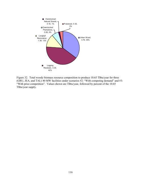
7. CONCLUSIONSIt is impossible to predict exactly what amount of which type of resources would beavailable to each facility at some price. However, under base case scenario #2, which assumesGRU, JEA, and TAL all use the biomass resources closest to them, the total amount of woodybiomass available for less than $3.00 per MMBtu delivered in the two-hour woodsheds of thethree facilities is 474,500 dry tons, or 7.20 TBtu, per year. Fifty-three percent of this total isurban wood waste within a two-hour haul of the three facilities, 37% is logging residues within a45-minute haul, and the remaining 10% is comprised of thinnings within a 30-minute haul. Thistotal includes 2.82 TBtu/year delivered to GRU, 2.56 TBtu/year to JEA, and 1.78 TBtu/yearTAL. The total consists of 11% of the wood waste, logging residues, and thinnings availablewithin a two-hour maximum haul of the three facilities.The least-cost biomass resources needed to provide 10.65 TBtu/year (enough to generatethree 40 MW facilities) in scenario #2 would be comprised of about 35% urban wood waste,42% logging residues, and about 20% from thinnings of natural stands and plantations. Toprovide 3.55 TBtu per year for each facility, the amount required to produce 40 MW, themarginal cost is expected to be $3.12, $3.23, and $3.25 per MMBtu at GRU, JEA, and TAL,respectively.About 3% of this least-cost supply of 10.65 TBtu/year would be met with nearby pulpwood(Figure 32). Pulpwood comprises 0%, 4%, and 6% of the least-cost resources used to provide 40MW for GRU, JEA, and TAL, respectively. The 10.65 TBtu/year needed to power these threefacilities, is 11% of the 100.91 TBtus/year from urban wood waste, logging residues, thinnings,and pulpwood identified within a two-hour haul of the three facilities. The resources included inthese scenarios are about 100%, 28%, 27%, 25%, 15%, and 0.4% of annually available urbanwood waste, logging resides, thinnings from longleaf pine restoration, thinnings fromoverstocked plantations, thinnings from overstocked natural stands, and pulpwood, respectively,within the two-hour one-way woodsheds, excluding overlap of adjacent woodsheds (Figure 33).115
OverstockedNatural Stands,0.16, 1% Pulpwood, 0.32,3%OverstockedPlantations,0.69, 6%LongleafRestoration,1.38, 13%Urban Wood,3.76, 35%LoggingResidues, 4.34,42%Figure 32. Total woody biomass resource composition to produce 10.65 TBtu/year for three(GRU, JEA, and TAL) 40 MW facilities under scenarios #2: “With competing demand” and #3:“With price competition”. Values shown are TBtu/year, followed by percent of the 10.65TBtu/year supply.116
Page 3 and 4:
ACKNOWLEDGEMENTSThe authors acknowl
Page 5 and 6:
4.2. Scenario A: Delivered to remot
Page 7:
Figure 22. Projected softwood and h
Page 10 and 11:
LIST OF ACRONYMS AND ABBREVIATIONSB
Page 12 and 13:
1. INTRODUCTION1.1. Project Backgro
Page 14 and 15:
Task-3: Transportation. Transportat
Page 16 and 17:
2. TASK 1: WOODSHED DELINEATION AND
Page 18 and 19:
calculations for urban wood waste a
Page 20 and 21:
the current pulpwood harvests are a
Page 22 and 23:
2,0001,800Acres (thousands)1,6001,4
Page 24 and 25:
ton -1 ($17.38 green ton -1 ) for t
Page 26 and 27:
$ per million BTU, delivered$4.00$3
Page 28 and 29:
10.65 TBtu/year required to meet de
Page 30 and 31:
haul time category in each county,
Page 32 and 33:
Figure 9. TAL Hopkins two-hour one-
Page 34 and 35:
Figure 11. GRU, JEA, and TAL woodsh
Page 36 and 37:
Dry tonsrecoverableTBtu/yearRecover
Page 38 and 39:
Dry tonsrecoverableTBtu/yearrecover
Page 40 and 41:
Table 6. Results for scenario #3,
Page 42 and 43:
Page 44 and 45:
Page 46 and 47:
6.005.004.00$/MMBtu3.002.001.001: W
Page 48 and 49:
Resource/haul time categoryDry tons
Page 50 and 51:
Page 52 and 53:
Page 54 and 55:
Page 56 and 57:
Page 58 and 59:
6.005.004.00$/MMBtu3.002.001.001: W
Page 60 and 61:
Page 62 and 63:
Page 64 and 65:
Page 66:
Page 69 and 70: Resource/haul time categoryDry tons
Page 71 and 72: 2.4.4. General resultsIt is difficu
Page 73 and 74: Table 22. Yield, acreage required,
Page 75 and 76: Table 25. Capital construction outp
Page 77 and 78: 3. TASK 2: SUSTAINABILITY IMPACTS F
Page 79 and 80: under this scenario are expected to
Page 81 and 82: acres in 1995 to 8.5 MM acres in 20
Page 83 and 84: 3.3. RESULTS3.3.1. GRUTable 27. Res
Page 85 and 86: 5.004.504.003.50$/MMBtu3.002.502.00
Page 87 and 88: Table 30. Results for the conservat
Page 89 and 90: 3.3.3. TAL Hopkins facilityTable 31
Page 91 and 92: 5.004.504.003.50$/MMBtu3.002.502.00
Page 93 and 94: For GRU most of these do not apply;
Page 95 and 96: Table 33. Concentration yard costs.
Page 97 and 98: location of the rail siding and the
Page 99 and 100: discussed, to get an idea of the pr
Page 101 and 102: 5. TASK 4: CO 2 EMISSIONS FROM HARV
Page 103 and 104: in fuel chips and the carbon in fue
Page 105 and 106: transporting coal. However, because
Page 107 and 108: 6. COMBINED RESOURCE AVAILABILITYPa
Page 109 and 110: Resource/haul time categoryTBtu/yea
Page 111 and 112: Table 39. Combined resources (resou
Page 117: Resource/haul time categoryTBtu/yea
Page 121 and 122: logging residues from 90% to 60% to
Page 123 and 124: ecommend that GRU, in coordination
Page 125: 9. REFERENCESBlack and Veach (2004)
show all

Biomass Resource Assessment Part I - Gainesville Regional Utilities

You also want an ePaper? Increase the reach of your titles

Delete template?

Save as template?