Book 2.indb - US Climate Change Science Program

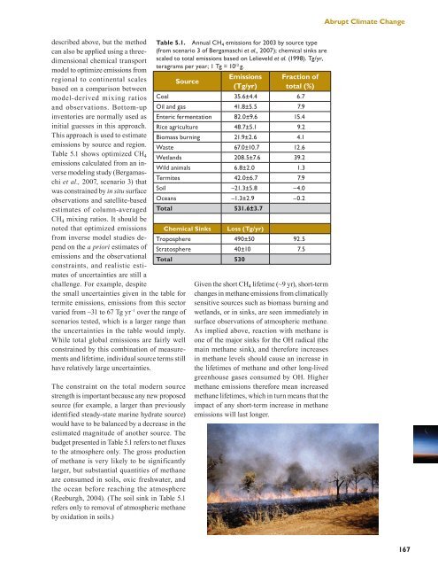
Abrupt Climate Changedescribed above, but the methodcan also be applied using a threedimensionalchemical transportmodel to optimize emissions fromregional to continental scalesbased on a comparison betweenmodel-derived mixing ratiosand observations. Bottom-upinventories are normally used asinitial guesses in this approach.This approach is used to estimateemissions by source and region.Table 5.1 shows optimized CH 4emissions calculated from an inversemodeling study (Bergamaschiet al., 2007, scenario 3) thatwas constrained by in situ surfaceobservations and satellite-basedestimates of column-averagedCH 4 mixing ratios. It should benoted that optimized emissionsfrom inverse model studies dependon the a priori estimates ofemissions and the observationalconstraints, and realistic estimatesof uncertainties are still achallenge. For example, despitethe small uncertainties given in the table fortermite emissions, emissions from this sectorvaried from ~31 to 67 Tg yr –1 over the range ofscenarios tested, which is a larger range thanthe uncertainties in the table would imply.While total global emissions are fairly wellconstrained by this combination of measurementsand lifetime, individual source terms stillhave relatively large uncertainties.The constraint on the total modern sourcestrength is important because any new proposedsource (for example, a larger than previouslyidentified steady-state marine hydrate source)would have to be balanced by a decrease in theestimated magnitude of another source. Thebudget presented in Table 5.1 refers to net fluxesto the atmosphere only. The gross productionof methane is very likely to be significantlylarger, but substantial quantities of methaneare consumed in soils, oxic freshwater, andthe ocean before reaching the atmosphere(Reeburgh, 2004). (The soil sink in Table 5.1refers only to removal of atmospheric methaneby oxidation in soils.)Table 5.1. Annual CH 4 emissions for 2003 by source type(from scenario 3 of Bergamaschi et al., 2007); chemical sinks arescaled to total emissions based on Lelieveld et al. (1998). Tg/yr,teragrams per year; 1 Tg = 10 12 g.SourceEmissions(Tg/yr)Fraction oftotal (%)Coal 35.6±4.4 6.7Oil and gas 41.8±5.5 7.9Enteric fermentation 82.0±9.6 15.4Rice agriculture 48.7±5.1 9.2Biomass burning 21.9±2.6 4.1Waste 67.0±10.7 12.6Wetlands 208.5±7.6 39.2Wild animals 6.8±2.0 1.3Termites 42.0±6.7 7.9Soil –21.3±5.8 –4.0Oceans –1.3±2.9 –0.2Total 531.6±3.7Chemical Sinks Loss (Tg/yr)Troposphere 490±50 92.5Stratosphere 40±10 7.5Total 530Given the short CH 4 lifetime (~9 yr), short-termchanges in methane emissions from climaticallysensitive sources such as biomass burning andwetlands, or in sinks, are seen immediately insurface observations of atmospheric methane.As implied above, reaction with methane isone of the major sinks for the OH radical (themain methane sink), and therefore increasesin methane levels should cause an increase inthe lifetimes of methane and other long-livedgreenhouse gases consumed by OH. Highermethane emissions therefore mean increasedmethane lifetimes, which in turn means that theimpact of any short-term increase in methaneemissions will last longer.167