WRF - Developmental Testbed Center

More documents

Recommendations

Info

Janjic, Z. I., 2000: Comments on “Development and Evaluation of a Convection Schemefor Use in Climate Models. J. Atmos. Sci., 57, p. 3686Janjic, Z. I., 2001: Nonsingular Implementation of the Mellor-Yamada Level 2.5 Schemein the NCEP Meso model. NCEP Office Note No. 437, 61 pp.Janjic, Z. I., 2002a: A Nonhydrostatic Model Based on a New Approach. EGS XVIII,Nice France, 21-26 April 2002.Janjic, Z. I., 2002b: Nonsingular Implementation of the Mellor–Yamada Level 2.5Scheme in the NCEP Meso model, NCEP Office Note, No. 437, 61 pp.Janjic, Z. I., 2003a: A Nonhydrostatic Model Based on a New Approach. Meteorologyand Atmospheric Physics, 82, 271-285. (Online: http://dx.doi.org/10.1007/s00703-001-0587-6).Janjic, Z. I., 2003b: The NCEP WRF Core and Further Development of Its PhysicalPackage. 5th International SRNWP Workshop on Non-Hydrostatic Modeling, Bad Orb,Germany, 27-29 October.Janjic, Z. I., 2004: The NCEP WRF Core. 12.7, Extended Abstract, 20th Conference onWeather Analysis and Forecasting/16th Conference on Numerical Weather Prediction,Seattle, WA, American Meteorological Society.Janjic, Z. I., J. P. Gerrity, Jr. and S. Nickovic, 2001: An Alternative Approach toNonhydrostatic Modeling. Mon. Wea. Rev., 129, 1164-1178.Janjic, Z. I., T. L. Black, E. Rogers, H. Chuang and G. DiMego, 2003: The NCEPNonhydrostatic Meso Model (NMM) and First Experiences with Its Applications.EGS/EGU/AGU Joint Assembly, Nice, France, 6-11 April.Janjic, Z. I, T. L. Black, E. Rogers, H. Chuang and G. DiMego, 2003: The NCEPNonhydrostatic Mesoscale Forecasting Model. 12.1, Extended Abstract, 10thConference on Mesoscale Processes, Portland, OR, American Meteorological Society.(Available Online).Kain J. S. and J. M. Fritsch, 1990: A One-Dimensional Entraining/Detraining PlumeModel and Its Application in Convective Parameterization. J. Atmos. Sci., 47, No. 23,pp. 2784–2802.Kain, J. S., and J. M. Fritsch, 1993: Convective parameterization for mesoscale models:The Kain-Fritcsh scheme, the representation of cumulus convection in numericalmodels, K. A. Emanuel and D.J. Raymond, Eds., Amer. Meteor. Soc., 246 pp.Kain J. S., 2004: The Kain–Fritsch Convective Parameterization: An Update. Journal ofApplied Meteorology, 43, No. 1, pp. 170–181.Kessler, E., 1969: On the distribution and continuity of water substance in atmosphericcirculation, Meteor. Monogr., 32, Amer. Meteor. Soc., 84 pp.Lacis, A. A., and J. E. Hansen, 1974: A parameterization for the absorption of solarradiation in the earth’s atmosphere. J. Atmos. Sci., 31, 118–133.Lin, Y.-L., R. D. Farley, and H. D. Orville, 1983: Bulk parameterization of the snow fieldin a cloud model. J. Climate Appl. Meteor., 22, 1065–1092.Miyakoda, K., and J. Sirutis, 1986: Manual of the E-physics. [Available fromGeophysical Fluid Dynamics Laboratory, Princeton University, P.O. Box 308,Princeton, NJ 08542]WRF-NMM V3: User’s Guide 5-35
Mlawer, E. J., S. J. Taubman, P. D. Brown, M. J. Iacono, and S. A. Clough, 1997:Radiative transfer for inhomogeneous atmosphere: RRTM, a validated correlated-kmodel for the longwave. J. Geophys. Res., 102 (D14), 16663–16682.Pan, H.-L. and W.-S. Wu, 1995: Implementing a Mass Flux Convection ParameterizationPackage for the NMC Medium-Range Forecast Model. NMC Office Note, No. 409,40pp. [Available from NCEP/EMC, W/NP2 Room 207, WWB, 5200 Auth Road,Washington, DC 20746-4304]Pan, H-L. and L. Mahrt, 1987: Interaction between soil hydrology and boundary layerdevelopments. Boundary Layer Meteor., 38, 185-202.Rutledge, S. A., and P. V. Hobbs, 1984: The mesoscale and microscale structure andorganization of clouds and precipitation in midlatitude cyclones. XII: A diagnosticmodeling study of precipitation development in narrow cloud-frontal rainbands. J.Atmos. Sci., 20, 2949–2972.Sadourny. R., 1975: The Dynamics of Finite-Difference Models of the Shallow-WaterEquations. J. Atmos. Sci., 32, No. 4, pp. 680–689.Schwarzkopf, M. D., and S. B. Fels, 1985: Improvements to the algorithm for computingCO2 transmissivities and cooling rates. J. Geophys. Res., 90, 541-550.Schwarzkopf, M. D., and S. B. Fels, 1991: The simplified exchange method revisited:An accurate, rapid method for computations of infrared cooling rates and fluxes. J.Geophys. Res., 96, 9075-9096.Skamarock, W. C., J. B. Klemp, J. Dudhia, D. O. Gill, D. M. Barker, W. Wang and J. G.Powers, 2005: A Description of the Advanced Research WRF Version 2, NCAR TechNote, NCAR/TN–468+STR, 88 pp. [Available from UCAR Communications, P.O. Box3000, Boulder, CO, 80307]. Available on-line at:http://box.mmm.ucar.edu/wrf/users/docs/arw_v2.pdf)Smirnova, T. G., J. M. Brown, and S. G. Benjamin, 1997: Performance of different soilmodel configurations in simulating ground surface temperature and surface fluxes.Mon. Wea. Rev., 125, 1870–1884.Smirnova, T. G., J. M. Brown, S. G. Benjamin, and D. Kim, 2000: Parameterization ofcold season processes in the MAPS land-surface scheme. J. Geophys. Res., 105 (D3),4077-4086.Tao, W.-K., J. Simpson, and M. McCumber 1989: An ice-water saturation adjustment,Mon. Wea. Rev., 117, 231–235.Troen, I. and L. Mahrt, 1986: A simple model of the atmospheric boundary layer:Sensitivity to surface evaporation. Boundary Layer Meteor., 37, 129-148.Thompson, G., R. M. Rasmussen, and K. Manning, 2004: Explicit forecasts of winterprecipitation using an improved bulk microphysics scheme. Part I: Description andsensitivity analysis. Mon. Wea. Rev., 132, 519–542.Wicker, L. J., and R. B. Wilhelmson, 1995: Simulation and analysis of tornadodevelopment and decay within a three-dimensional supercell thunderstorm. J. Atmos.Sci., 52, 2675–2703.WRF-NMM V3: User’s Guide 5-36
Page 1 and 2: ForewordUser's Guide for the NMM Co
Page 3 and 4: • WPP Directory Structure 7-3•
Page 5 and 6: The WRF modeling system software is
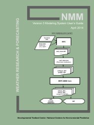
Page 7 and 8: WRF-NMM FLOW CHARTTerrestrialDataMo
Page 9 and 10: Vendor Hardware OS CompilerCray X1
Page 11 and 12: If all of these executables are def
Page 13 and 14: Once the tar file is obtained, gunz
Page 15 and 16: HWRF is set, then (3) will be autom
Page 17 and 18: In addition to these three links, a
Page 19 and 20: • Real-data simulations• Non-hy
Page 21 and 22: k. Morrison double-moment scheme (1
Page 23 and 24: g. GFDL surface layer (88): (This s
Page 25 and 26: Other physics optionsa. gwd_opt: Gr
Page 27 and 28: to the convergence of meridians app
Page 29 and 30: Variable NamesValue(Example)Descrip
Page 39 and 40: mpirun.lsf wrf.exeand for interacti
Page 41 and 42: The boundary conditions for the nes
Page 43 and 44: Examples:1. One nest and one level
Page 45 and 46: ottom_top_stag = 28 ;soil_layers_st
Page 47 and 48: float HLENSW(Time, south_north, wes
Page 49 and 50: float HBOTS(Time, south_north, west
Page 51: operational mesoscale Eta model. J.
Page 55 and 56: NCEP WRF Postprocessor (WPP)WPP Int
Page 57 and 58: ./configureYou will be given a list
Page 59 and 60: equested output field. If the pre-r
Page 61 and 62: RAINCV SNOW HBOTRAINNCVSNOWCNote: F
Page 63 and 64: Running WPPFour scripts for running
Page 65 and 66: i. As the grid id of a pre-defined
Page 67 and 68: The GrADS package is available from
Page 69 and 70: Height on pressure surface HEIGHT O
Page 71 and 72: MELTPrecipitation type (4 types) -
Page 73 and 74: Press at tropopause PRESS AT TROPOP
Page 75 and 76: RIP4RIP IntroductionRIP (which stan
Page 77 and 78: A successful compilation will resul
Page 79 and 80: iinterp = 0v v v v vH V H V h h h h
Page 81 and 82: espectively, of the centered domain
Page 83 and 84: This can be either 'h' (for hours),
Page 85: eal variable expect values that are
Page 88 and 89: of all the requested trajectories a
Page 90 and 91: Creating Vis5D Dataset with RIPVis5
Page 92 and 93: User’s Guide for the NMM Core of
Page 94 and 95: Configuration: The configure script
Page 96 and 97: This program reads the contents of
Page 98 and 99: Period - Describes communications f
Page 100 and 101: fine grid), f (forcing, how the lat
Page 102 and 103:
# halo HALO_NMM_K dyn_nmm8:q2;24:t
Page 104 and 105:
(http://www.mmm.ucar.edu/wrf/WG2/Ti
Page 106 and 107:
User's Guide for the NMM Core of th
Page 108 and 109:
2. Make sure the files listed below
Page 110 and 111:
User's Guide for the NMM Core of th
Page 112 and 113:
Program geogridThe purpose of geogr
Page 114 and 115:
1. Define a model coarse domain and
Page 116 and 117:
to GEOGRID.TBL in the geogrid direc
Page 118 and 119:
the GRIB data were downloaded to th
Page 120 and 121:
By this point, there is generally n
Page 122 and 123:
two nests are defined to have the s
Page 124 and 125:
Note: For the WRF-NMM the variables
Page 126 and 127:
simulations may use a constant SST
Page 128 and 129:
entire simulation domain, and data
Page 130 and 131:
that lists the variables and attrib
Page 132 and 133:
http://www.ecmwf.int/products/data/
Page 134 and 135:
intermediate formats (metgrid/src/r
Page 136 and 137:
GRIB1| Level| From | To |Param| Typ
Page 138 and 139:
corresponding source grid point. Gi
Page 140 and 141:
tile_x = 1200tile_y = 1200tile_z =
Page 142 and 143:
1. PARENT_ID : A list of MAX_DOM in
Page 144 and 145:
V -DX- H| / |DY dx DY| / |H - DX- V
Page 146 and 147:
intermediate files if ungrib is to
Page 148 and 149:
the index and data tiles for the da
Page 150 and 151:
1. PROJECTION : A character string
Page 152 and 153:
25. SCALE_FACTOR : A real value tha
Page 154 and 155:
10. INTERP_MASK : The name of the f
Page 156 and 157:
1. four_pt : Four-point bi-linear i
Page 158 and 159:
8. search : Breadth-first search in
Page 160 and 161:
19 Mixed Tundra20 Barren TundraTabl
Page 162 and 163:
LU_INDEX:units = "category" ;LU_IND
Page 164 and 165:
netcdf met_em.d01.2009-01-05_12:00:
Page 166:
}:ISOILWATER = 14 ;:grid_id = 1 ;:p
show all

WRF - Developmental Testbed Center

Create successful ePaper yourself

Delete template?

Save as template?