The Art of Practical and Precise Strain Based ... - Webprofile.info

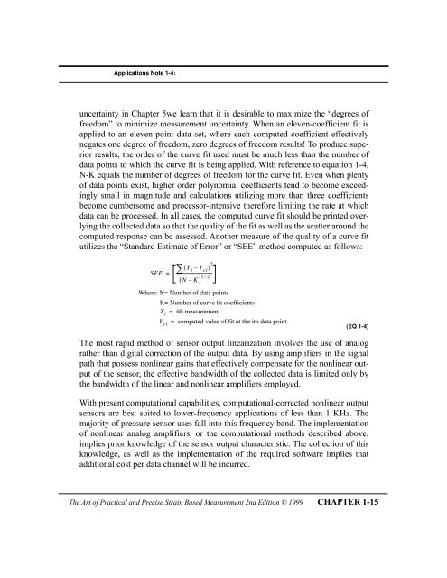
Applications Note 1-4:uncertainty in Chapter 5we learn that it is desirable to maximize the Òdegrees offreedomÓ to minimize measurement uncertainty. When an eleven-coefficient fit isapplied to an eleven-point data set, where each computed coefficient effectivelynegates one degree of freedom, zero degrees of freedom results! To produce superiorresults, the order of the curve fit used must be much less than the number ofdata points to which the curve fit is being applied. With reference to equation 1-4,N-K equals the number of degrees of freedom for the curve fit. Even when plentyof data points exist, higher order polynomial coefficients tend to become exceedinglysmall in magnitude and calculations utilizing more than three coefficientsbecome cumbersome and processor-intensive therefore limiting the rate at whichdata can be processed. In all cases, the computed curve fit should be printed overlyingthe collected data so that the quality of the fit as well as the scatter around thecomputed response can be assessed. Another measure of the quality of a curve fitutilizes the ÒStandard Estimate of ErrorÓ or ÒSEEÓ method computed as follows:SEE =å ( Y i Ð Y-------------------------------- ci( N Ð K) Where: N= Number of data pointsK= Number of curve fit coefficientsY i = ith measurementY ci = computed value of fit at the ith data point(EQ 1-4)The most rapid method of sensor output linearization involves the use of analograther than digital correction of the output data. By using amplifiers in the signalpath that possess nonlinear gains that effectively compensate for the nonlinear outputof the sensor, the effective bandwidth of the collected data is limited only bythe bandwidth of the linear and nonlinear amplifiers employed.With present computational capabilities, computational-corrected nonlinear outputsensors are best suited to lower-frequency applications of less than 1 KHz. Themajority of pressure sensor uses fall into this frequency band. The implementationof nonlinear analog amplifiers, or the computational methods described above,implies prior knowledge of the sensor output characteristic. The collection of thisknowledge, as well as the implementation of the required software implies thatadditional cost per data channel will be incurred.The Art of Practical and Precise Strain Based Measurement 2nd Edition © 1999 CHAPTER 1-15