THÈSE Koléhè Abdoulaye COULIBALY-PASQUIER

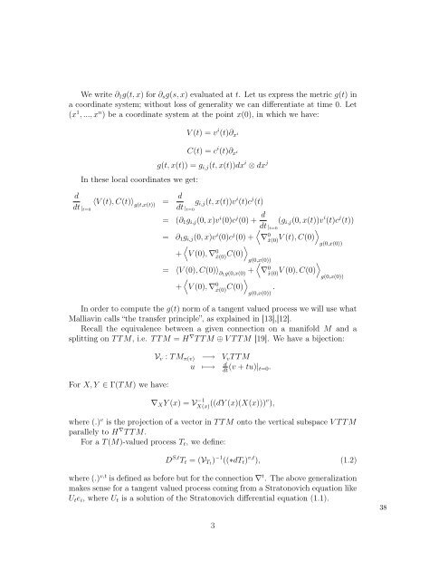
We write ∂ 1 g(t, x) for ∂ s g(s, x) evaluated at t. Let us express the metric g(t) ina coordinate system; without loss of generality we can differentiate at time 0. Let(x 1 , ..., x n ) be a coordinate system at the point x(0), in which we have:V (t) = v i (t)∂ x iIn these local coordinates we get:C(t) = c i (t)∂ x ig(t, x(t)) = g i,j (t, x(t))dx i ⊗ dx jddt | t=0〈V (t), C(t)〉 g(t,x(t))= d dt | t=0g i,j (t, x(t))v i (t)c j (t)= (∂ 1 g i,j (0, x)v i (0)c j (0) + d (g i,j (0, x(t))v i (t)c j (t))dt | t=0 〉= ∂ 1 g i,j (0, x)v i (0)c j (0) +〈∇ 0 ẋ(0)〉V (t), C(0) g(0,x(0))+〈V (0), ∇ 0 ẋ(0) C(0) g(0,x(0)) 〈〉= 〈V (0), C(0)〉 ∂1 g(0,x(0) + ∇ 0 ẋ(0)〉V (0), C(0) g(0,x(0))+〈V (0), ∇ 0 ẋ(0) C(0) .g(0,x(0))In order to compute the g(t) norm of a tangent valued process we will use whatMalliavin calls “the transfer principle”, as explained in [13],[12].Recall the equivalence between a given connection on a manifold M and asplitting on T T M, i.e. T T M = H ∇ T T M ⊕ V T T M [19]. We have a bijection:For X, Y ∈ Γ(T M) we have:V v : T M π(v) −→ V v T T Mu ↦−→ d (v + tu)| dt t=0.∇ X Y (x) = V −1X(x) ((dY (x)(X(x)))v ),where (.) v is the projection of a vector in T T M onto the vertical subspace V T T Mparallely to H ∇ T T M.For a T (M)-valued process T t , we define:D S,t T t = (V Tt ) −1 ((∗dT t ) v,t ), (1.2)where (.) v,t is defined as before but for the connection ∇ t . The above generalizationmakes sense for a tangent valued process coming from a Stratonovich equation likeU t e i , where U t is a solution of the Stratonovich differential equation (1.1).383