THÈSE Koléhè Abdoulaye COULIBALY-PASQUIER

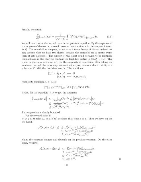
Finally, we obtain:∂∂t | t=t 0ρ t (x, y) =12ρ t0 (x, y)∫ 10〈 ˙γ t 0(s), ˙γ t 0(s)〉 ∂∂t |t=t 0g(t)ds. (3.1)We will now control the second term in the previous equation. By the exponentialconvergence of the metric, we could assume that the time is in the compact interval[0, 1]. The manifold is compact, so we have a finite family of charts (indeed, wemay assume that we have two charts, because the manifold has a metric whichturns it into a sphere). The support of this chart could be taken to be relativelycompact, and in this chart we can take the Euclidien metric i.e 〈∂ i , ∂ j 〉 E = δ j i . Thisis not in general a metric on M. For the simplicity of expression, after taking theminimum over all charts we may assume that we just have one chart. Let S 1 be asphere in R n with the Euclidean metric. The functional:reaches its minimum C > 0, so:[0, 1] × S 1 × M −→ R(t, v, x) ↦−→ g ij (t, x)v i v j‖T ‖ E ≤ C −1 ‖T ‖ g(t) , ∀t ∈ [0, 1], ∀T ∈ T M.Hence, for the equation (3.1) we get the estimate:∣ ∂ | ∫ ∣1∂t t=t 0ρ t (x, y) ∣ ≤2ρ t0 (x,y) C1 e −δt 0 1 ∣0∣〈 ˙γ t 0(s), ˙γ t 0 ∣∣ds(s)〉 E∫ 1≤2ρ t0 (x,y) C1 (C) −1 e −δt 0 1 ∣0∣〈 ˙γ t 0(s), ˙γ t 0∣(s)〉 g(t0 ) ∣ds≤ 1 2 C1 (C) −1 e −δt 0.This expression is clearly bounded.For the second point ii),let x, y ∈ M take γ ∞ be a g(∞)-geodesic that joins x to y. Then we have, on theone hand,ρ 2 t (x, y) − ρ 2 ∞(x, y) ≤ ∫ 1〈 ˙γ 0 ∞(s), ˙γ ∞ (s)〉 g(t)−g(∞) ds≤ Cste ∫ −δt 1‖ ˙γ 0 ∞(s)‖ 2 g(∞) ds≤ Cste −δt diam 2 g(∞) (M);where the constant changes and depends on the previous constant. On the otherhand, we have:ρ 2 ∞(x, y) − ρ 2 t (x, y) ≤ ∫ 1〈 0 ˙γt (s), ˙γ t (s)〉 g(∞)−g(t) ds≤ Cste ∫ −δt 1‖ 0 ˙γt (s)‖ 2 g(t) ds≤ Cste −δt diam 2 g(t) (M)≤ cst 1 e −δt ,8116