THÈSE Koléhè Abdoulaye COULIBALY-PASQUIER

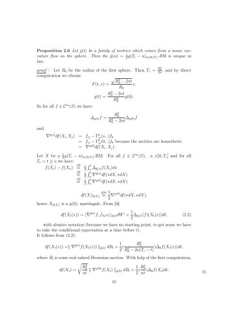
Proposition 2.6 Let g(t) be a family of metrics which comes from a mean curvatureflow on the sphere. Then the ˜g(u) = 1g(T 2 c − u) u∈]0,Tc]-BM is unique inlaw.proof : Let R 0 be the radius of the first sphere. Then T c = R2 0, and by direct2ncomputation we obtain:√R2F (t, x) = 0 − 2ntx,R 0So for all f ∈ C ∞ (S) we have:g(t) = R2 0 − 2ntg(0).R02and∆ g(t) f =R 2 0R 2 0 − 2nt ∆ g(0)f∇ g(s) df(X i , X j ) = f ij − Γ k ij(s, .)f k= f ij − Γ k ij(0, .)f k because the metrics are homothetic= ∇ g(0) df(X i , X j ).Let X be a 1g(T 2 c − u) u∈]0,Tc]-BM. For all f ∈ C ∞ (S), u ∈]0, T c ] and for allT c > t ≥ u we have:M ∫f(X t ) − f(X u ) ≡1 t ∆˜g(s)f(X 2 u s )dsM ∫≡1 t ∇˜g(s) df(∗dX, ∗dX)2 u∫ tu ∇g(0) df(∗dX, ∗dX)M≡12dM 1df(X) ]0,Tc] ≡2 ∇g(0) df(∗dX, ∗dX),hence X ]0,Tc] is a g(0)- martingale. From [4]:df(X t (x)) = 〈∇˜g(t) f, / 0,t v i 〉˜g(t) dW i + 1 2 ∆˜g(t)(f)(X t (x))dt, (2.2)with abusive notation (because we have no starting point, to get sense we haveto take the conditional expectation at a time before t).It follows from (2.2):df(X t (x)) =‖ ∇˜g(t) f(X t (x)) ‖˜g(t) dB t + 1 2 ( R 2 0R 2 0 − 2n(T c − t) )∆ 0f(X t (x))dt,where B t is some real-valued Brownian motion. With help of the first computation,df(X t ) =√R20nt ‖ ∇g(0) f(X t ) ‖ g(0) dB t + 1 2 (R2 0nt )∆ 0f(X t )dt.7510