- Page 1 and 2:
Roadside Revegetation An Integrated
- Page 3 and 4:
Roadside Revegetation: An Integrate
- Page 5 and 6:
TABLE OF CONTENTS 3— Initiation P
- Page 7 and 8:
TABLE OF CONTENTS 5.9 Pests 127 5.9
- Page 9 and 10:
TABLE OF CONTENTS 10.4 Post Install
- Page 11 and 12:
TABLE OF CONTENTS Figure 3-5 | Exam
- Page 13 and 14:
TABLE OF CONTENTS Figure 6-10 | Cas
- Page 15 and 16:
TABLE OF CONTENTS Figure 10-91 | Se
- Page 17 and 18:
TABLE OF CONTENTS Insets Inset 2-1
- Page 19 and 20:
PREFACE In 1998, the Western Federa
- Page 21 and 22:
INTRODUCTION 1— Introduction 1.1
- Page 23 and 24:
INTRODUCTION 15 to 20 percent of th
- Page 25 and 26:
INTRODUCTION and others 2016, and c
- Page 27 and 28:
INTRODUCTION ◾◾ Integrate goals
- Page 29 and 30:
INTRODUCTION 1.5.2 WHAT ARE NATIVE
- Page 31 and 32:
INTRODUCTION Figure 1-9 | Roadside
- Page 33 and 34:
INTRODUCTION 1.6.1 INITIATION OVERV
- Page 35 and 36:
INITIATION PART ONE: COOPERATORS AN
- Page 37 and 38:
INITIATION PART ONE: COOPERATORS AN
- Page 39 and 40:
INITIATION PART ONE: COOPERATORS AN
- Page 41 and 42:
INITIATION PART ONE: COOPERATORS AN
- Page 43 and 44:
INITIATION PART ONE: COOPERATORS AN
- Page 45 and 46:
INITIATION PART TWO: ROAD PLANS AND
- Page 47 and 48:
INITIATION PART TWO: ROAD PLANS AND
- Page 49 and 50:
INITIATION PART TWO: ROAD PLANS AND
- Page 51 and 52:
INITIATION PART TWO: ROAD PLANS AND
- Page 53 and 54:
INITIATION PART TWO: ROAD PLANS AND
- Page 55 and 56:
PLANNING PHASE ONE: ORIENT 4— Pla
- Page 57 and 58:
PLANNING PHASE ONE: ORIENT Once rev
- Page 59 and 60:
PLANNING PHASE ONE: ORIENT Revegeta
- Page 61 and 62:
PLANNING PHASE ONE: ORIENT site on
- Page 63 and 64:
PLANNING PHASE ONE: ORIENT The info
- Page 65 and 66:
PLANNING PHASE ONE: ORIENT Figure 4
- Page 67 and 68:
PLANNING PHASE ONE: ORIENT Figure 4
- Page 69 and 70:
PLANNING PHASE ONE: ORIENT Disturbe
- Page 71 and 72:
PLANNING PHASE ONE: ORIENT Table 4-
- Page 73 and 74:
PLANNING PHASE ONE: ORIENT Column H
- Page 75 and 76:
PLANNING PHASE ONE: ORIENT species
- Page 77 and 78:
PLANNING PHASE TWO: ASSESS SITE 5.1
- Page 79 and 80:
PLANNING PHASE TWO: ASSESS SITE 5.2
- Page 81 and 82:
PLANNING PHASE TWO: ASSESS SITE dur
- Page 83 and 84:
PLANNING PHASE TWO: ASSESS SITE Mit
- Page 85 and 86:
PLANNING PHASE TWO: ASSESS SITE Mit
- Page 87 and 88:
PLANNING PHASE TWO: ASSESS SITE Sta
- Page 89 and 90:
PLANNING PHASE TWO: ASSESS SITE cry
- Page 91 and 92:
PLANNING PHASE TWO: ASSESS SITE pen
- Page 93 and 94:
PLANNING PHASE TWO: ASSESS SITE 5.3
- Page 95 and 96:
PLANNING PHASE TWO: ASSESS SITE Mit
- Page 97 and 98:
PLANNING PHASE TWO: ASSESS SITE Min
- Page 99 and 100:
PLANNING PHASE TWO: ASSESS SITE Rel
- Page 101 and 102:
PLANNING PHASE TWO: ASSESS SITE 5.4
- Page 103 and 104:
PLANNING PHASE TWO: ASSESS SITE 5.4
- Page 105 and 106:
PLANNING PHASE TWO: ASSESS SITE bac
- Page 107 and 108:
PLANNING PHASE TWO: ASSESS SITE Org
- Page 109 and 110:
PLANNING PHASE TWO: ASSESS SITE ind
- Page 111 and 112:
PLANNING PHASE TWO: ASSESS SITE Ins
- Page 113 and 114:
PLANNING PHASE TWO: ASSESS SITE soi
- Page 115 and 116:
PLANNING PHASE TWO: ASSESS SITE Fig
- Page 117 and 118:
PLANNING PHASE TWO: ASSESS SITE Mit
- Page 119 and 120:
PLANNING PHASE TWO: ASSESS SITE Hig
- Page 121 and 122:
PLANNING PHASE TWO: ASSESS SITE oft
- Page 123 and 124:
PLANNING PHASE TWO: ASSESS SITE Mit
- Page 125 and 126:
PLANNING PHASE TWO: ASSESS SITE 5.6
- Page 127 and 128:
PLANNING PHASE TWO: ASSESS SITE 5.6
- Page 129 and 130:
PLANNING PHASE TWO: ASSESS SITE ang
- Page 131 and 132:
PLANNING PHASE TWO: ASSESS SITE Mit
- Page 133 and 134:
PLANNING PHASE TWO: ASSESS SITE Slo
- Page 135 and 136:
PLANNING PHASE TWO: ASSESS SITE 5.7
- Page 137 and 138:
PLANNING PHASE TWO: ASSESS SITE Wat
- Page 139 and 140:
PLANNING PHASE TWO: ASSESS SITE the
- Page 141 and 142:
క క క క క క PLANNING PH
- Page 143 and 144:
PLANNING PHASE TWO: ASSESS SITE cle
- Page 145 and 146:
PLANNING PHASE TWO: ASSESS SITE bum
- Page 147 and 148:
PLANNING PHASE TWO: ASSESS SITE nit
- Page 149 and 150:
PLANNING PHASE TWO: ASSESS SITE Pla
- Page 151 and 152:
PLANNING PHASE TWO: ASSESS SITE 5.9
- Page 153 and 154:
PLANNING PHASE TWO: ASSESS SITE Fig
- Page 155 and 156:
PLANNING PHASE TWO: ASSESS SITE 5.1
- Page 157 and 158:
PLANNING PHASE THREE: VEGETATION AN
- Page 159 and 160:
PLANNING PHASE THREE: VEGETATION AN
- Page 161 and 162:
PLANNING PHASE THREE: VEGETATION AN
- Page 163 and 164:
PLANNING PHASE THREE: VEGETATION AN
- Page 165 and 166:
PLANNING PHASE THREE: VEGETATION AN
- Page 167 and 168:
PLANNING PHASE THREE: VEGETATION AN
- Page 169 and 170:
PLANNING PHASE THREE: VEGETATION AN
- Page 171 and 172:
PLANNING PHASE THREE: VEGETATION AN
- Page 173 and 174:
PLANNING PHASE FOUR: INTEGRATE AND
- Page 175 and 176:
PLANNING PHASE FOUR: INTEGRATE AND
- Page 177 and 178:
క క క క క క క క క
- Page 179 and 180:
PLANNING PHASE FOUR: INTEGRATE AND
- Page 181 and 182:
REVEGETATION PLAN EXAMPLE PREFACE T
- Page 183 and 184:
REVEGETATION PLAN EXAMPLE TABLE OF
- Page 185 and 186:
REVEGETATION PLAN EXAMPLE BACKGROUN
- Page 187 and 188:
REVEGETATION PLAN EXAMPLE BACKGROUN
- Page 189 and 190:
REVEGETATION PLAN EXAMPLE REVEGETAT
- Page 191 and 192:
REVEGETATION PLAN EXAMPLE REVEGETAT
- Page 193 and 194:
REVEGETATION PLAN EXAMPLE REVEGETAT
- Page 195 and 196:
REVEGETATION PLAN EXAMPLE REVEGETAT
- Page 197 and 198:
REVEGETATION PLAN EXAMPLE REVEGETAT
- Page 199 and 200:
REVEGETATION PLAN EXAMPLE REVEGETAT
- Page 201 and 202:
REVEGETATION PLAN EXAMPLE REVEGETAT
- Page 203 and 204:
REVEGETATION PLAN EXAMPLE NON-NATIV
- Page 205 and 206:
REVEGETATION PLAN EXAMPLE SUCCESS C
- Page 207 and 208:
REVEGETATION PLAN EXAMPLE APPROXIMA
- Page 209 and 210:
REVEGETATION PLAN EXAMPLE APPROXIMA
- Page 211 and 212:
REVEGETATION PLAN EXAMPLE APPROXIMA
- Page 213 and 214:
REVEGETATION PLAN EXAMPLE APPENDIX
- Page 215 and 216:
REVEGETATION PLAN EXAMPLE APPENDIX
- Page 217 and 218:
REVEGETATION PLAN EXAMPLE APPENDIX
- Page 219 and 220:
REVEGETATION PLAN EXAMPLE APPENDIX
- Page 221 and 222:
REVEGETATION PLAN EXAMPLE APPENDIX
- Page 223 and 224:
REVEGETATION PLAN EXAMPLE APPENDIX
- Page 225 and 226:
REVEGETATION PLAN EXAMPLE REFERENCE
- Page 227 and 228:
REVEGETATION PLAN EXAMPLE REFERENCE
- Page 229 and 230:
IMPLEMENTATION 9.1 INTRODUCTION A s
- Page 231 and 232:
IMPLEMENTATION 9.3 REVIEW TREATMENT
- Page 233 and 234:
IMPLEMENTATION 9.4 DEVELOP CONTRACT
- Page 235 and 236:
IMPLEMENTATION 9.6 EXAMPLE STATEMEN
- Page 237 and 238:
IMPLEMENTATION an active role in pr
- Page 239 and 240:
IMPLEMENTATION addressed environmen
- Page 241 and 242:
IMPLEMENTATION GUIDES 10— Impleme
- Page 243 and 244:
IMPLEMENTATION GUIDES 10.1.1 FERTIL
- Page 245 and 246:
IMPLEMENTATION GUIDES Areas adjacen
- Page 247 and 248:
IMPLEMENTATION GUIDES Table 10.2 |
- Page 249 and 250:
IMPLEMENTATION GUIDES The nutrient
- Page 251 and 252:
IMPLEMENTATION GUIDES nutrient stra
- Page 253 and 254:
IMPLEMENTATION GUIDES Fertilizer In
- Page 255 and 256:
IMPLEMENTATION GUIDES amendments, l
- Page 257 and 258:
IMPLEMENTATION GUIDES A general rul
- Page 259 and 260:
IMPLEMENTATION GUIDES 10.1.3 MULCHE
- Page 261 and 262:
IMPLEMENTATION GUIDES permeable or
- Page 263 and 264:
IMPLEMENTATION GUIDES and straw fro
- Page 265 and 266:
IMPLEMENTATION GUIDES mulch. If the
- Page 267 and 268:
IMPLEMENTATION GUIDES To avoid this
- Page 269 and 270:
IMPLEMENTATION GUIDES control, stra
- Page 271 and 272:
IMPLEMENTATION GUIDES (often less t
- Page 273 and 274:
IMPLEMENTATION GUIDES most topsoil
- Page 275 and 276:
IMPLEMENTATION GUIDES Table 10.6 |
- Page 277 and 278:
IMPLEMENTATION GUIDES 10.1.5 ORGANI
- Page 279 and 280:
IMPLEMENTATION GUIDES rock fragment
- Page 281 and 282:
IMPLEMENTATION GUIDES Table 10.8 |
- Page 283 and 284:
IMPLEMENTATION GUIDES Carbon-to-Nit
- Page 285 and 286:
IMPLEMENTATION GUIDES be broadened
- Page 287 and 288:
IMPLEMENTATION GUIDES Therefore, le
- Page 289 and 290:
IMPLEMENTATION GUIDES compaction an
- Page 291 and 292:
IMPLEMENTATION GUIDES Pure Culture
- Page 293 and 294:
IMPLEMENTATION GUIDES ◾◾ Design
- Page 295 and 296:
IMPLEMENTATION GUIDES Table 10.11 |
- Page 297 and 298:
IMPLEMENTATION GUIDES can be used.
- Page 299 and 300:
IMPLEMENTATION GUIDES harvesting, s
- Page 301 and 302:
IMPLEMENTATION GUIDES In Figure 10-
- Page 303 and 304:
IMPLEMENTATION GUIDES of the seed i
- Page 305 and 306:
IMPLEMENTATION GUIDES is conducted
- Page 307 and 308:
IMPLEMENTATION GUIDES Project Name
- Page 309 and 310:
IMPLEMENTATION GUIDES variety of sp
- Page 311 and 312:
IMPLEMENTATION GUIDES Inset 10-14 |
- Page 313 and 314:
IMPLEMENTATION GUIDES Table 10.13 |
- Page 315 and 316:
IMPLEMENTATION GUIDES Installation
- Page 317 and 318:
IMPLEMENTATION GUIDES Special Treat
- Page 319 and 320:
IMPLEMENTATION GUIDES Determine Tra
- Page 321 and 322:
IMPLEMENTATION GUIDES to the surfac
- Page 323 and 324:
IMPLEMENTATION GUIDES year, the see
- Page 325 and 326:
IMPLEMENTATION GUIDES Table 10.14 |
- Page 327 and 328:
IMPLEMENTATION GUIDES ◾◾ Minimu
- Page 329 and 330:
IMPLEMENTATION GUIDES debris are se
- Page 331 and 332:
IMPLEMENTATION GUIDES A B Figure 10
- Page 333 and 334:
IMPLEMENTATION GUIDES Table 10.15 |
- Page 335 and 336:
IMPLEMENTATION GUIDES production-or
- Page 337 and 338:
IMPLEMENTATION GUIDES Restoration s
- Page 339 and 340:
IMPLEMENTATION GUIDES ◾◾ Approp
- Page 341 and 342:
IMPLEMENTATION GUIDES Unbalanced or
- Page 343 and 344:
IMPLEMENTATION GUIDES You can get a
- Page 345 and 346:
IMPLEMENTATION GUIDES Inset 10-18 |
- Page 347 and 348:
IMPLEMENTATION GUIDES planters stan
- Page 349 and 350:
IMPLEMENTATION GUIDES uniformity is
- Page 351 and 352:
IMPLEMENTATION GUIDES Seed drills c
- Page 353 and 354:
IMPLEMENTATION GUIDES Each species
- Page 355 and 356:
IMPLEMENTATION GUIDES would have lo
- Page 357 and 358:
IMPLEMENTATION GUIDES seeds. Poorly
- Page 359 and 360:
IMPLEMENTATION GUIDES ◾◾ Some s
- Page 361 and 362:
IMPLEMENTATION GUIDES Consideration
- Page 363 and 364:
IMPLEMENTATION GUIDES (1979) found
- Page 365 and 366:
IMPLEMENTATION GUIDES Revegetation
- Page 367 and 368:
IMPLEMENTATION GUIDES ◾◾ Storag
- Page 369 and 370:
IMPLEMENTATION GUIDES During the hy
- Page 371 and 372:
IMPLEMENTATION GUIDES (Pezeshki and
- Page 373 and 374: IMPLEMENTATION GUIDES Inset 10-22 |
- Page 375 and 376: IMPLEMENTATION GUIDES inch) of soil
- Page 377 and 378: IMPLEMENTATION GUIDES determine the
- Page 379 and 380: IMPLEMENTATION GUIDES A B Figure 10
- Page 381 and 382: IMPLEMENTATION GUIDES minimize the
- Page 383 and 384: IMPLEMENTATION GUIDES Planting - Pr
- Page 385 and 386: IMPLEMENTATION GUIDES not secured w
- Page 387 and 388: IMPLEMENTATION GUIDES ◾◾ High s
- Page 389 and 390: IMPLEMENTATION GUIDES 10.4.5 IRRIGA
- Page 391 and 392: IMPLEMENTATION GUIDES of water, the
- Page 393 and 394: IMPLEMENTATION GUIDES Placing a pre
- Page 395 and 396: INTRODUCTION MONITORING AND MANAGEM
- Page 397 and 398: MONITORING AND MANAGEMENT Monitorin
- Page 399 and 400: క క క క క క క క క
- Page 401 and 402: MONITORING AND MANAGEMENT ◾◾ Mo
- Page 403 and 404: MONITORING AND MANAGEMENT Analysis
- Page 405 and 406: INTRODUCTION MONITORING PROCEDURES
- Page 407 and 408: MONITORING PROCEDURES ◾◾ Rectil
- Page 409 and 410: MONITORING PROCEDURES 1 2 3 4 5 6 7
- Page 411 and 412: MONITORING PROCEDURES Use of a digi
- Page 413 and 414: MONITORING PROCEDURES 1 2 3 4 5 6 7
- Page 415 and 416: MONITORING PROCEDURES ◾◾ Rectil
- Page 417 and 418: MONITORING PROCEDURES N w e E 14.6
- Page 419 and 420: MONITORING PROCEDURES Sampling of D
- Page 421 and 422: MONITORING PROCEDURES Using the equ
- Page 423: MONITORING PROCEDURES 12.9 STATISTI
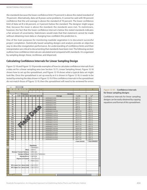
- Page 427 and 428: MONITORING PROCEDURES Calculating C
- Page 429 and 430: MONITORING PROCEDURES that if more
- Page 431 and 432: MONITORING PROCEDURES 1 2 3 4 5 6 7
- Page 433 and 434: MONITORING PROCEDURES bee counts ca
- Page 435 and 436: POLLINATOR-SPECIFIC CASE STUDIES Ch
- Page 437 and 438: POLLINATOR-SPECIFIC CASE STUDIES pr
- Page 439 and 440: BIBLIOGRAPHY Alexander R. 2003a. A
- Page 441 and 442: BIBLIOGRAPHY Bower AD, St. Clair JB
- Page 443 and 444: BIBLIOGRAPHY Claassen VP, Zasoski R
- Page 445 and 446: BIBLIOGRAPHY Dyer K, Curtis L, Will
- Page 447 and 448: BIBLIOGRAPHY Greaves RD, Hermann RK
- Page 449 and 450: BIBLIOGRAPHY (Available at: https:/
- Page 451 and 452: BIBLIOGRAPHY Landis T, Tinus RW, Mc
- Page 453 and 454: BIBLIOGRAPHY Miller RM, May SW. 197
- Page 455 and 456: BIBLIOGRAPHY between biodiversity c
- Page 457 and 458: BIBLIOGRAPHY Soil Survey Staff. 197
- Page 459 and 460: BIBLIOGRAPHY Trent A, Nolte D, Wagn
- Page 461 and 462: BIBLIOGRAPHY Wolf DD, Blaser RE, Mo
- Page 464: APPENDIX Native Revegetation Plants
- Page 468: APPENDIX Native Revegetation Plants
- Page 472: APPENDIX Native Revegetation Plants
- Page 476:
APPENDIX Native Revegetation Plants
- Page 480:
APPENDIX Native Revegetation Plants
- Page 484:
APPENDIX Native Revegetation Plants
- Page 488:
APPENDIX Native Revegetation Plants
- Page 492:
APPENDIX IOWA — NATIVE REVEGETATI
- Page 496:
APPENDIX Iowa — Native Revegetati
- Page 500:
APPENDIX Iowa — Native Revegetati
- Page 504:
APPENDIX Iowa — Native Revegetati
- Page 508:
APPENDIX Iowa — Native Revegetati
- Page 512:
APPENDIX Kansas — Native Revegeta
- Page 516:
APPENDIX Kansas — Native Revegeta
- Page 520:
APPENDIX Kansas — Native Revegeta
- Page 524:
APPENDIX Kansas — Native Revegeta
- Page 528:
APPENDIX Kansas — Native Revegeta
- Page 532:
APPENDIX Minnesota — Native Reveg
- Page 536:
APPENDIX Minnesota — Native Reveg
- Page 540:
APPENDIX Minnesota — Native Reveg
- Page 544:
APPENDIX Minnesota — Native Reveg
- Page 548:
APPENDIX Missouri — Native Revege
- Page 552:
APPENDIX Missouri — Native Revege
- Page 556:
APPENDIX Missouri — Native Revege
- Page 560:
APPENDIX Missouri — Native Revege
- Page 564:
APPENDIX Missouri — Native Revege
- Page 568:
APPENDIX Missouri — Native Revege
- Page 572:
APPENDIX Oklahoma — Native Revege
- Page 576:
APPENDIX Oklahoma — Native Revege
- Page 580:
APPENDIX Oklahoma — Native Revege
- Page 584:
APPENDIX Oklahoma — Native Revege
- Page 588:
APPENDIX TEXAS — NATIVE REVEGETAT
- Page 592:
APPENDIX Texas — Native Revegetat
- Page 596:
APPENDIX Texas — Native Revegetat
- Page 600:
APPENDIX Texas — Native Revegetat
- Page 604:
APPENDIX Texas — Native Revegetat