ST 520 Statistical Principles of Clinical Trials - NCSU Statistics ...

More documents

Recommendations

Info

CHAPTER 8 ST 520, A. TSIATIS and D. Zhang 8 Causality, Non-compliance and Intent-to-treat 8.1 Causality and Counterfactual Random Variables Throughout the course, we’ve repeatedly said that randomization allows us to make causal statements regarding the effect of treatment on the primary response of interest. In this section, we will be more formal. The actual definition of cause and effect has been hotly debated over the years especially by philosophers. We will take a particular point of view using what are called counterfactual random variables. As usual, we consider a super-population of individuals that we are interested in and assume that the participants in a clinical trial represent a random sample from this population. For concreteness, let us consider a clinical trial which will compare a new treatment (treatment 1) to no treatment or placebo (treatment 0). We define the counterfactual random variable Y ∗ 1 to denote the response (may be a binary or continuous outcome) that a randomly selected individual from our population if, possibly contrary to fact, that individual received treatment 1 (new treatment). Similarly, we define the counterfactual random variable Y ∗ 0 to denote the response that a randomly selected individual from our population if, possibly contrary to fact, that individual received treatment 0 (placebo). We imagine the existence of both random variables (Y ∗ 0 ∗ , Y ) even though in actuality it would be impossible to observe both responses on any given individual. Thus the term counterfactual or “contrary to fact”. At the individual level, we say that treatment causes the effect Y ∗ 1 − Y ∗ 0 . Clearly, if an individual knew their response to both treatment and placebo, then he/she would choose whichever gave the better response. Of course, this is not possible at the individual level but perhaps we can look at this question at the population level. That is, we will consider the population mean causal effect; namely ∆ = E(Y ∗ 1 −Y ∗ 0 1 ∗ ∗ ) = E(Y ) −E(Y ). If ∆ is positive, then on average the response on treatment 1 will be better than on treatment 0. At the individual level this will not necessarily imply that any specific individual will be guaranteed to benefit, but on average, the population as a whole will benefit. Knowledge of the average causal effect at the population level, if it can be obtained or estimated, is still useful at the individual level. Say, for example, it has been proved that ∆ is positive; i.e. that on average treatment 1 is better than treatment 0, then in the absence of any additional a-priori knowledge that would distinguish one individual from the other, the best treatment choice for any PAGE 118 1 0
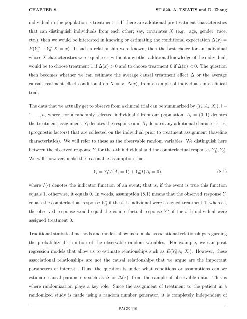
CHAPTER 8 ST 520, A. TSIATIS and D. Zhang individual in the population is treatment 1. If there are additional pre-treatment characteristics that can distinguish individuals from each other; say, covariates X (e.g. age, gender, race, etc.), then we would be interested in knowing or estimating the conditional expectation ∆(x) = E(Y ∗ 1 ∗ − Y0 |X = x). If such a relationship were known, then the best choice for an individual whose X characteristics were equal to x, without any other additional knowledge of the individual, would be to choose treatment 1 if ∆(x) > 0 and to choose treatment 0 if ∆(x) < 0. The question then becomes whether we can estimate the average causal treatment effect ∆ or the average causal treatment effect conditional on X = x, ∆(x), from a sample of individuals in a clinical trial. The data that we actually get to observe from a clinical trial can be summarized by (Yi, Ai, Xi), i = 1, . . .,n, where, for a randomly selected individual i from our population, Ai = (0, 1) denotes the treatment assignment, Yi denotes the response and Xi denotes any additional characteristics, (prognostic factors) that are collected on the individual prior to treatment assignment (baseline characteristics). We will refer to these as the observable random variables. We distinguish here between the observed response Yi for the i-th individual and the counterfactual responses Y ∗ ∗ 1i , Y0i . We will, however, make the reasonable assumption that Yi = Y ∗ 1iI(Ai = 1) + Y ∗ 0iI(Ai = 0), (8.1) where I(·) denotes the indicator function of an event; that is, if the event is true this function equals 1, otherwise, it equals 0. In words, assumption (8.1) means that the observed response Yi equals the counterfactual response Y ∗ 1i if the i-th individual were assigned treatment 1; whereas, the observed response would equal the counterfactual response Y ∗ 0i if the i-th individual were assigned treatment 0. Traditional statistical methods and models allow us to make associational relationships regarding the probability distribution of the observable random variables. For example, we can posit regression models that allow us to estimate relationships such as E(Yi|Ai, Xi). However, these associational relationships are not the causal relationships that we argue are the important parameters of interest. Thus, the question is under what conditions or assumptions can we estimate causal parameters such as ∆ or ∆(x), from the sample of observable data. This is where randomization plays a key role. Since the assignment of treatment to the patient in a randomized study is made using a random number generator, it is completely independent of PAGE 119
Page 1 and 2:
ST 520 Statistical Principles of Cl
Page 3 and 4:
TABLE OF CONTENTS ST 520, A. Tsiati
Page 5 and 6:
CHAPTER 1 ST 520, A. TSIATIS and D.
Page 7 and 8:
Page 9 and 10:
Page 11 and 12:
Page 13 and 14:
Page 15 and 16:
Page 17 and 18:
Page 19 and 20:
Page 21 and 22:
Page 23 and 24:
Page 25 and 26:
Page 27 and 28:
Page 29 and 30:
Page 31 and 32:
Page 33 and 34:
Page 35 and 36:
Page 37 and 38:
Page 39 and 40:
Page 41 and 42:
Page 43 and 44:
Page 45 and 46:
Page 47 and 48:
Page 49 and 50:
Page 51 and 52:
Page 53 and 54:
Page 55 and 56:
Page 57 and 58:
Page 59 and 60:
Page 61 and 62:
Page 63 and 64:
Page 65 and 66:
Page 67 and 68:
Page 69 and 70:
Page 71 and 72: CHAPTER 4 ST 520, A. TSIATIS and D.
Page 121: CHAPTER 7 ST 520, A. TSIATIS and D.
Page 169 and 170: CHAPTER 10 ST 520, A. TSIATIS and D
Page 171 and 172: CHAPTER 10 ST 520, A. TSIATIS and D
Page 173 and 174:
CHAPTER 10 ST 520, A. TSIATIS and D
Page 175 and 176:
Page 177 and 178:
Page 179 and 180:
Page 181 and 182:
Page 183 and 184:
Page 185 and 186:
Page 187 and 188:
Page 189 and 190:
Page 191 and 192:
Page 193 and 194:
Page 195 and 196:
Page 197 and 198:
Page 199 and 200:
show all

ST 520 Statistical Principles of Clinical Trials - NCSU Statistics ...

Create successful ePaper yourself

Delete template?

Save as template?