ST 520 Statistical Principles of Clinical Trials - NCSU Statistics ...

CHAPTER 10 ST 520, A. TSIATIS and D. Zhang
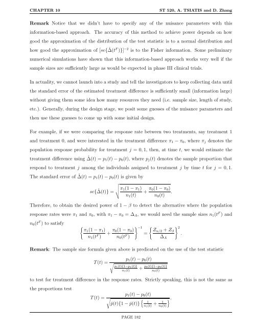
Remark Notice that we didn’t have to specify any of the nuisance parameters with this
information-based approach. The accuracy of this method to achieve power depends on how
good the approximation of the distribution of the test statistic is to a normal distribution and
how good the approximation of [se{ ˆ ∆(t F )}] −2 is to the Fisher information. Some preliminary
numerical simulations have shown that this information-based approach works very well if the
sample sizes are sufficiently large as would be expected in phase III clinical trials.
In actuality, we cannot launch into a study and tell the investigators to keep collecting data until
the standard error of the estimated treatment difference is sufficiently small (information large)
without giving them some idea how many resources they need (i.e. sample size, length of study,
etc.). Generally, during the design stage, we posit some guesses of the nuisance parameters and
then use these guesses to come up with some initial design.
For example, if we were comparing the response rate between two treatments, say treatment 1
and treatment 0, and were interested in the treatment difference π1 − π0, where πj denotes the
population response probability for treatment j = 0, 1, then, at time t, we would estimate the
treatment difference using ˆ ∆(t) = p1(t) − p0(t), where pj(t) denotes the sample proportion that
respond to treatment j among the individuals assigned to treatment j by time t for j = 0, 1.
The standard error of ˆ ∆(t) = p1(t) − p0(t) is given by
se{ ˆ �
�
�
∆(t)} = �π1(1 − π1)
n1(t) + π0(1 − π0)
.
n0(t)
Therefore, to obtain the desired power of 1 − β to detect the alternative where the population
response rates were π1 and π0, with π1 − π0 = ∆A, we would need the sample sizes n1(t F ) and
n0(t F ) to satisfy
�
π1(1 − π1)
n1(tF ) + π0(1 − π0)
n0(tF �−1 =
)
� Zα/2 + Zβ
Remark: The sample size formula given above is predicated on the use of the test statistic
T(t) =
p1(t) − p0(t)
� p1(t){1−p1(t)}
n1(t)
∆A
+ p0(t){1−p0(t)}
n0(t)
to test for treatment difference in the response rates. Strictly speaking, this is not the same as
the proportions test
T(t) =
p1(t) − p0(t)
�
¯p(t){1 − ¯p(t)} � 1 1 + n1(t) n0(t)
PAGE 182
�,
� 2
.