ST 520 Statistical Principles of Clinical Trials - NCSU Statistics ...
ST 520 Statistical Principles of Clinical Trials - NCSU Statistics ...
ST 520 Statistical Principles of Clinical Trials - NCSU Statistics ...

You also want an ePaper? Increase the reach of your titles
YUMPU automatically turns print PDFs into web optimized ePapers that Google loves.
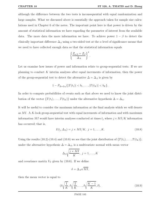
CHAPTER 10 <strong>ST</strong> <strong>520</strong>, A. TSIATIS and D. Zhang<br />
although the difference between the two tests is inconsequential with equal randomization and<br />
large samples. What we discussed above is essentially the approach taken for sample size calcu-<br />
lations used in Chapter 6 <strong>of</strong> the notes. The important point here is that power is driven by the<br />
amount <strong>of</strong> statistical information we have regarding the parameter <strong>of</strong> interest from the available<br />
data. The more data the more information we have. To achieve power 1 − β to detect the<br />
clinically important difference ∆A using a two-sided test at the α level <strong>of</strong> significance means that<br />
we need to have collected enough data so that the statistical information equals<br />
� Zα/2 + Zβ<br />
∆A<br />
Let us examine how issues <strong>of</strong> power and information relate to group-sequential tests. If we are<br />
planning to conduct K interim analyses after equal increments <strong>of</strong> information, then the power<br />
� 2<br />
.<br />
<strong>of</strong> the group-sequential test to detect the alternative ∆ = ∆A is given by<br />
1 − P∆=∆A {|T(t1)| < b1, . . .,|T(tK)| < bK}.<br />
In order to compute probabilities <strong>of</strong> events such as that above we need to know the joint distri-<br />
bution <strong>of</strong> the vector {T(t1), . . .,T(tK)} under the alternative hypothesis ∆ = ∆A.<br />
It will be useful to consider the maximum information at the final analysis which we will denote<br />
as MI. A K-look group-sequential test with equal increments <strong>of</strong> information and with maximum<br />
information MI would have interim analyses conducted at times tj where j ×MI/K information<br />
has occurred; that is,<br />
I(tj, ∆A) = j × MI/K, j = 1, . . .,K. (10.8)<br />
Using the results (10.2)-(10.4) and (10.8) we see that the joint distribution <strong>of</strong> {T(t1), . . .,T(tK)},<br />
under the alternative hypothesis ∆ = ∆A, is a multivariate normal with mean vector<br />
�<br />
j × MI<br />
∆A , j = 1, . . .,K<br />
K<br />
and covariance matrix VT given by (10.6). If we define<br />
√<br />
δ = ∆A MI,<br />
then the mean vector is equal to<br />
� � �<br />
1 2 K − 1<br />
(δ , δ , . . .,δ , δ). (10.9)<br />
K K K<br />
PAGE 183