ST 520 Statistical Principles of Clinical Trials - NCSU Statistics ...

CHAPTER 9 ST 520, A. TSIATIS and D. Zhang
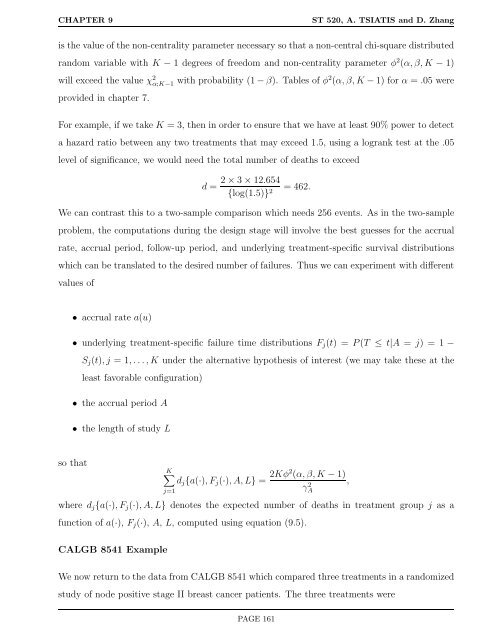
is the value of the non-centrality parameter necessary so that a non-central chi-square distributed
random variable with K − 1 degrees of freedom and non-centrality parameter φ 2 (α, β, K − 1)
will exceed the value χ 2 α;K−1 with probability (1 − β). Tables of φ2 (α, β, K − 1) for α = .05 were
provided in chapter 7.
For example, if we take K = 3, then in order to ensure that we have at least 90% power to detect
a hazard ratio between any two treatments that may exceed 1.5, using a logrank test at the .05
level of significance, we would need the total number of deaths to exceed
d =
2 × 3 × 12.654
= 462.
{log(1.5)} 2
We can contrast this to a two-sample comparison which needs 256 events. As in the two-sample
problem, the computations during the design stage will involve the best guesses for the accrual
rate, accrual period, follow-up period, and underlying treatment-specific survival distributions
which can be translated to the desired number of failures. Thus we can experiment with different
values of
• accrual rate a(u)
• underlying treatment-specific failure time distributions Fj(t) = P(T ≤ t|A = j) = 1 −
Sj(t), j = 1, . . .,K under the alternative hypothesis of interest (we may take these at the
least favorable configuration)
• the accrual period A
• the length of study L
so that
K�
j=1
dj{a(·), Fj(·), A, L} = 2Kφ2 (α, β, K − 1)
γ2 ,
A
where dj{a(·), Fj(·), A, L} denotes the expected number of deaths in treatment group j as a
function of a(·), Fj(·), A, L, computed using equation (9.5).
CALGB 8541 Example
We now return to the data from CALGB 8541 which compared three treatments in a randomized
study of node positive stage II breast cancer patients. The three treatments were
PAGE 161