ST 520 Statistical Principles of Clinical Trials - NCSU Statistics ...

CHAPTER 10 ST 520, A. TSIATIS and D. Zhang
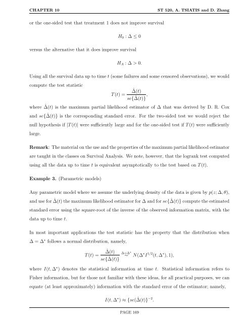
or the one-sided test that treatment 1 does not improve survival
H0 : ∆ ≤ 0
versus the alternative that it does improve survival
HA : ∆ > 0.
Using all the survival data up to time t (some failures and some censored observations), we would
compute the test statistic
T(t) = ˆ ∆(t)
se{ ˆ ∆(t)} ,
where ˆ ∆(t) is the maximum partial likelihood estimator of ∆ that was derived by D. R. Cox
and se{ ˆ ∆(t)} is the corresponding standard error. For the two-sided test we would reject the
null hypothesis if |T(t)| were sufficiently large and for the one-sided test if T(t) were sufficiently
large.
Remark: The material on the use and the properties of the maximum partial likelihood estimator
are taught in the classes on Survival Analysis. We note, however, that the logrank test computed
using all the data up to time t is equivalent asymptotically to the test based on T(t).
Example 3. (Parametric models)
Any parametric model where we assume the underlying density of the data is given by p(z; ∆, θ),
and use for ˆ ∆(t) the maximum likelihood estimator for ∆ and for se{ ˆ ∆(t)} compute the estimated
standard error using the square-root of the inverse of the observed information matrix, with the
data up to time t.
In most important applications the test statistic has the property that the distribution when
∆ = ∆ ∗ follows a normal distribution, namely,
T(t) = ˆ ∆(t)
se{ ˆ ∆=∆
∆(t)}
∗
∼ N(∆ ∗ I 1/2 (t, ∆ ∗ ), 1),
where I(t, ∆ ∗ ) denotes the statistical information at time t. Statistical information refers to
Fisher information, but for those not familiar with these ideas, for all practical purposes, we can
equate (at least approximately) information with the standard error of the estimator; namely,
I(t, ∆ ∗ ) ≈ {se( ˆ ∆(t)} −2 .
PAGE 169