Through-Wall Imaging With UWB Radar System - KEMT FEI TUKE

2.5 Radar Imaging Methods Overview 16
equations based methods. Very good subdivision of the basic imaging methods
into these two categories is shown in [79].
• Backprojection Algorithms: This class of algorithms contains the conventional
SAR imaging (geometrical migration) as well as simple migration algorithms
as diffraction summation.
• Backpropagation Algorithms: This class of algorithms contains most migration
algorithms (including the well known Kirchoff migration) as well as the
wave equation based, non-conventional SAR.
The first migration methods are based on a geometrical approach. After the
introduction of computers, more complex techniques based on the scalar wave
equation were introduced. A good overview of these techniques is given in [150,17].
2.5.2 SAR Imaging - Geometrical Migration
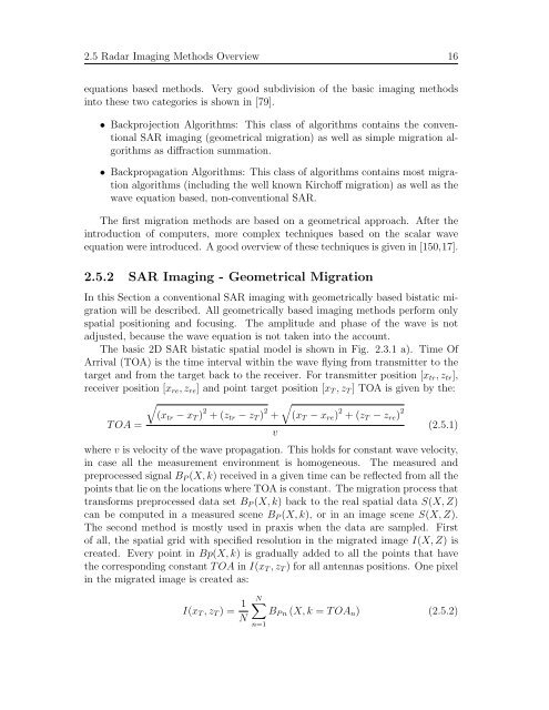
In this Section a conventional SAR imaging with geometrically based bistatic migration
will be described. All geometrically based imaging methods perform only
spatial positioning and focusing. The amplitude and phase of the wave is not
adjusted, because the wave equation is not taken into the account.
The basic 2D SAR bistatic spatial model is shown in Fig. 2.3.1 a). Time Of
Arrival (TOA) is the time interval within the wave flying from transmitter to the
target and from the target back to the receiver. For transmitter position [xtr, ztr],
receiver position [xre, zre] and point target position [xT , zT ] TOA is given by the:
T OA =
�
(xtr − xT ) 2 + (ztr − zT ) 2 +
v
�
(xT − xre) 2 + (zT − zre) 2
(2.5.1)
where v is velocity of the wave propagation. This holds for constant wave velocity,
in case all the measurement environment is homogeneous. The measured and
preprocessed signal BP (X, k) received in a given time can be reflected from all the
points that lie on the locations where TOA is constant. The migration process that
transforms preprocessed data set BP (X, k) back to the real spatial data S(X, Z)
can be computed in a measured scene BP (X, k), or in an image scene S(X, Z).
The second method is mostly used in praxis when the data are sampled. First
of all, the spatial grid with specified resolution in the migrated image I(X, Z) is
created. Every point in Bp(X, k) is gradually added to all the points that have
the corresponding constant T OA in I(xT , zT ) for all antennas positions. One pixel
in the migrated image is created as:
I(xT , zT ) = 1
N
N�
BP n (X, k = T OAn) (2.5.2)
n=1