Through-Wall Imaging With UWB Radar System - KEMT FEI TUKE
Through-Wall Imaging With UWB Radar System - KEMT FEI TUKE
Through-Wall Imaging With UWB Radar System - KEMT FEI TUKE

You also want an ePaper? Increase the reach of your titles
YUMPU automatically turns print PDFs into web optimized ePapers that Google loves.
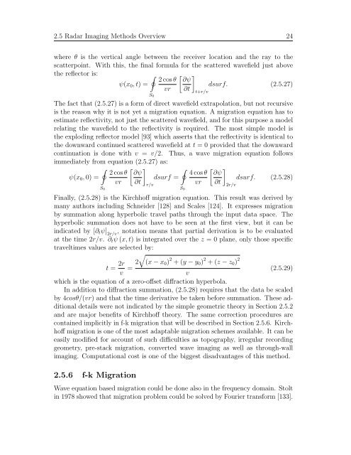
2.5 <strong>Radar</strong> <strong>Imaging</strong> Methods Overview 24<br />
where θ is the vertical angle between the receiver location and the ray to the<br />
scatterpoint. <strong>With</strong> this, the final formula for the scattered wavefield just above<br />
the reflector is:<br />
� � �<br />
2 cos θ ∂ψ<br />
ψ(x0, t) =<br />
dsurf. (2.5.27)<br />
vr ∂t t+r/v<br />
S0<br />
The fact that (2.5.27) is a form of direct wavefield extrapolation, but not recursive<br />
is the reason why it is not yet a migration equation. A migration equation has to<br />
estimate reflectivity, not just the scattered wavefield, and for this purpose a model<br />
relating the wavefield to the reflectivity is required. The most simple model is<br />
the exploding reflector model [93] which asserts that the reflectivity is identical to<br />
the downward continued scattered wavefield at t = 0 provided that the downward<br />
continuation is done with v = v/2. Thus, a wave migration equation follows<br />
immediately from equation (2.5.27) as:<br />
� � �<br />
�<br />
2 cos θ ∂ψ<br />
ψ(x0, 0) =<br />
dsurf =<br />
vr ∂t<br />
S0<br />
r/v<br />
S0<br />
4 cos θ<br />
vr<br />
� �<br />
∂ψ<br />
dsurf. (2.5.28)<br />
∂t 2r/v<br />
Finally, (2.5.28) is the Kirchhoff migration equation. This result was derived by<br />
many authors including Schneider [128] and Scales [124]. It expresses migration<br />
by summation along hyperbolic travel paths through the input data space. The<br />
hyperbolic summation does not have to be seen at the first view, but it can be<br />
indicated by [∂tψ] 2r/v , notation means that partial derivation is to be evaluated<br />
at the time 2r/v. ∂tψ (x, t) is integrated over the z = 0 plane, only those specific<br />
traveltimes values are selected by:<br />
t = 2r<br />
�<br />
2 (x − x0)<br />
= 2 + (y − y0) 2 + (z − z0) 2<br />
(2.5.29)<br />
v<br />
which is the equation of a zero-offset diffraction hyperbola.<br />
In addition to diffraction summation, (2.5.28) requires that the data be scaled<br />
by 4cosθ/(vr) and that the time derivative be taken before summation. These additional<br />
details were not indicated by the simple geometric theory in Section 2.5.2<br />
and are major benefits of Kirchhoff theory. The same correction procedures are<br />
contained implicitly in f-k migration that will be described in Section 2.5.6. Kirchhoff<br />
migration is one of the most adaptable migration schemes available. It can be<br />
easily modified for account of such difficulties as topography, irregular recording<br />
geometry, pre-stack migration, converted wave imaging as well as through-wall<br />
imaging. Computational cost is one of the biggest disadvantages of this method.<br />
2.5.6 f-k Migration<br />
Wave equation based migration could be done also in the frequency domain. Stolt<br />
in 1978 showed that migration problem could be solved by Fourier transform [133].<br />
v