Through-Wall Imaging With UWB Radar System - KEMT FEI TUKE

2.5 Radar Imaging Methods Overview 20
2.5.5 Kirchhoff Migration
Kirchhoff migration is based on solving scalar wave equation. Partial differential
equations called separation of variables based on Green’s theorem are used to solve
this scalar wave equation [96]. Kirchhoff migration theory provides a detailed
prescription for computing the amplitude and phase along the wavefront, and in
variable velocity, the shape of the wavefront. Kirchhoff theory shows that the
summation along the hyperbola must be done with specific weights. In this case,
the hyperbola is replaced by a more general shape.
Kirchhoff migration is mathematically complicated algorithm and is described
in depth in e.g. [96] and [150] and applied for landmine detection e.g. in [57].
In this section, only a short overview of mathematical description from [96] with
focus on physical interpretation of the method is explained.
Gauss’s theorem [59] and Green’s theorem [23] is used for Kirchhoff migration
description. Gauss’s theorem generalizes the basic integral result (2.5.11) into the
more dimensions (2.5.12).
�b
a
φ ′ (x)dx = φ(x) � �b a = φ(b) − φ(a) (2.5.11)
�
V
�∇. � �
Advol =
∂V
�A.�ndsurf (2.5.12)
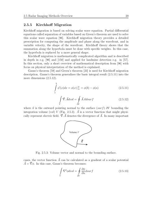
where �n is the outward pointing normal to the surface (surf) ∂V bounding the
integration volume (vol) V (Fig. 2.5.3). � A is a vector function that might physically
represent electric field. � ∇. � A denotes the divergence of � A. In many important
Volume V
Fig. 2.5.3: Volume vector and normal to the bounding surface.
cases, the vector function � A can be calculated as a gradient of a scalar potential
�A = � ∇φ. In this case, Gauss’s theorem becomes:
�
∇ 2 �
∂φ
φdvol = dsurf (2.5.13)
∂n
V
∂V
n