Through-Wall Imaging With UWB Radar System - KEMT FEI TUKE
Through-Wall Imaging With UWB Radar System - KEMT FEI TUKE
Through-Wall Imaging With UWB Radar System - KEMT FEI TUKE

You also want an ePaper? Increase the reach of your titles
YUMPU automatically turns print PDFs into web optimized ePapers that Google loves.
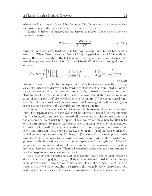
2.5 <strong>Radar</strong> <strong>Imaging</strong> Methods Overview 22<br />
where the δ (x0 − x) is a Dirac delta function. The Green’s function describes how<br />
the wave changes during travel from point x0 to the point x.<br />
Kirchhoff diffraction integral can be derived as follows. Let ψ be a solution to<br />
the scalar wave equation:<br />
∇ 2 ψ (x, t) = 1<br />
v2 ∂2ψ (x, t)<br />
∂2t (2.5.21)<br />
where ψ (x, t) is a wave function, v is the wave velocity and do not has to be a<br />
constant. When Green’s theorem from (2.5.18) is applied to the (2.5.21) with the<br />
aid of Helmholtz equation, Hankel functions, and good mathematical skills (the<br />
complete process can be find in [96]) the Kirchhoff’s diffraction integral can be<br />
obtained:<br />
�<br />
ψ(x0, t) =<br />
∂V<br />
�<br />
1<br />
r<br />
� �<br />
∂ψ<br />
−<br />
∂n t+r/v0<br />
1 ∂r<br />
v0r ∂n<br />
� �<br />
∂ψ<br />
+<br />
∂t t+r/v0<br />
1<br />
r2 ∂r<br />
∂n [ψ] �<br />
dsurf<br />
t+r/v0<br />
(2.5.22)<br />
where r = |x − x0|, x0 is the source position and v0 is a constant velocity. In many<br />
cases this integral is derived for forward modeling with the result that all of the<br />
terms are evaluated at the retarded time t − r/v0 instead of the advanced time.<br />
This Kirchhoff diffraction integral expresses the wavefield at the observation point<br />
xo at time t in terms of the wavefield on the boundary ∂V at the advanced time<br />
t + r/v0. It is known from Fourier theory that knowledge of both ψ and ∂nψ is<br />
necessary to reconstruct the wavefield at any internal point.<br />
In order to obtain practical migration formula, two essential tasks are required.<br />
First, the apparent need to know ∂nψ must be addressed. Second, the requirement<br />
that the integration surface must extend all the way around the volume containing<br />
the observation point must be dropped. There are various ways how to fulfill both<br />
of these arguments. Schneider [128] solved the requirement of ∂nψ by using a dipole<br />
Green’s function with an image source above the recording place, that vanished at<br />
z = 0 and cancelled the ∂nψ term in (2.5.22). Wiggins in [143] adapted Schneider’s<br />
technique to rough topography. Docherty in [51] showed that a monopole Green’s<br />
can also leads to an acceptable result and once again challenged Schneider’s argument,<br />
so the integral over the infinite hemisphere could be neglected. After all,<br />
migration by summation along diffraction curves or by wavefront superposition<br />
has been done for many years. Though Schneider’s derivation has been criticized,<br />
his final expressions are considered correct.<br />
As a first step in adapting (2.5.22) it is usually considered as appropriate to<br />
discard the term 1 1<br />
r2 ∂r<br />
∂n [ψ(x)] . This is called the near-field term and decays<br />
t+r/v0<br />
more strongly with r than the other two terms. Then, the surface S = ∂V will be<br />
taken as the z = 0 plane, S0, plus the surface infinitesimally below the reflector, Sz,<br />
and finally these surfaces will be joined at infinity by vertical cylindrical walls, S∞,