Through-Wall Imaging With UWB Radar System - KEMT FEI TUKE
Through-Wall Imaging With UWB Radar System - KEMT FEI TUKE
Through-Wall Imaging With UWB Radar System - KEMT FEI TUKE
Create successful ePaper yourself
Turn your PDF publications into a flip-book with our unique Google optimized e-Paper software.
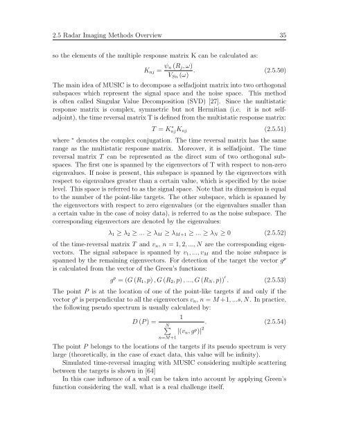
2.5 <strong>Radar</strong> <strong>Imaging</strong> Methods Overview 35<br />
so the elements of the multiple response matrix K can be calculated as:<br />
Knj = ψn (Rj, ω)<br />
. (2.5.50)<br />
VSn (ω)<br />
The main idea of MUSIC is to decompose a selfadjoint matrix into two orthogonal<br />
subspaces which represent the signal space and the noise space. This method<br />
is often called Singular Value Decomposition (SVD) [27]. Since the multistatic<br />
response matrix is complex, symmetric but not Hermitian (i.e. it is not selfadjoint),<br />
the time reversal matrix T is defined from the multistatic response matrix:<br />
T = K ∗ njKnj<br />
(2.5.51)<br />
where ∗ denotes the complex conjugation. The time reversal matrix has the same<br />
range as the multistatic response matrix. Moreover, it is selfadjoint. The time<br />
reversal matrix T can be represented as the direct sum of two orthogonal subspaces.<br />
The first one is spanned by the eigenvectors of T with respect to non-zero<br />
eigenvalues. If noise is present, this subspace is spanned by the eigenvectors with<br />
respect to eigenvalues greater than a certain value, which is specified by the noise<br />
level. This space is referred to as the signal space. Note that its dimension is equal<br />
to the number of the point-like targets. The other subspace, which is spanned by<br />
the eigenvectors with respect to zero eigenvalues (or the eigenvalues smaller than<br />
a certain value in the case of noisy data), is referred to as the noise subspace. The<br />
corresponding eigenvectors are denoted by the eigenvalues:<br />
λ1 ≥ λ2 ≥ ... ≥ λM ≥ λM+1 ≥ ... ≥ λN ≥ 0 (2.5.52)<br />
of the time-reversal matrix T and vn, n = 1, 2, ..., N are the corresponding eigenvectors.<br />
The signal subspace is spanned by v1, ..., vM and the noise subspace is<br />
spanned by the remaining eigenvectors. For detection of the target the vector g p<br />
is calculated from the vector of the Green’s functions:<br />
g p = (G (R1, p) , G (R2, p) , ..., G (RN, p)) ′ . (2.5.53)<br />
The point P is at the location of one of the point-like targets if and only if the<br />
vector gp is perpendicular to all the eigenvectors vn, n = M +1, ...s, N. In practice,<br />
the following pseudo spectrum is usually calculated by:<br />
1<br />
D (P ) =<br />
N�<br />
|(vn, gp )| 2<br />
. (2.5.54)<br />
n=M+1<br />
The point P belongs to the locations of the targets if its pseudo spectrum is very<br />
large (theoretically, in the case of exact data, this value will be infinity).<br />
Simulated time-reversal imaging with MUSIC considering multiple scattering<br />
between the targets is shown in [64]<br />
In this case influence of a wall can be taken into account by applying Green’s<br />
function considering the wall, what is a real challenge itself.


