Upscaling and Inverse Modeling of Groundwater Flow and Mass ...

82 CHAPTER 4. MODELING TRANSIENT GROUNDWATER . . .
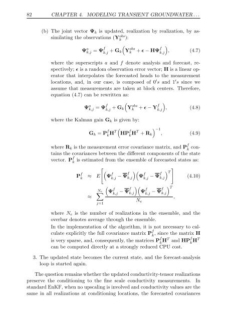
(b) The joint vector Ψk is updated, realization by realization, by assimilating
the observations (Y obs
k ):
Ψ a k,j
= Ψf
k,j + Gk
(
Y obs
k + ϵ − HΨf k,j
)
, (4.7)
where the superscripts a and f denote analysis and forecast, respectively;
ϵ is a random observation error vector; H is a linear operator
that interpolates the forecasted heads to the measurement
locations, and, in our case, is composed of 0 ′ s and 1 ′ s since we
assume that measurements are taken at block centers. Therefore,
equation (4.7) can be rewritten as:
Ψ a k,j
= Ψf
k,j + Gk
where the Kalman gain Gk is given by:
(
Y obs
k + ϵ − Yf
k,j
)
, (4.8)
Gk = P f
(
kHT HP f
kHT ) −1
+ Rk , (4.9)
where Rk is the measurement error covariance matrix, and P f
k con-
tains the covariances between the different components of the state
vector. P f
k is estimated from the ensemble of forecasted states as:
P f
[
(
k ≈ E Ψ f
)(
k,j − Ψfk,j
Ψ f
]
) T
k,j − Ψfk,j
(4.10)
≈
Ne ∑
j=1
(
Ψ f
)(
k,j − Ψfk,j
Ψ f
) T
k,j − Ψfk,j
where Ne is the number of realizations in the ensemble, and the
overbar denotes average through the ensemble.
In the implementation of the algorithm, it is not necessary to calculate
explicitly the full covariance matrix P f
k , since the matrix H
is very sparse, and, consequently, the matrices P f
kHT and HP f
kHT can be computed directly at a strongly reduced CPU cost.
3. The updated state becomes the current state, and the forecast-analysis
loop is started again.
The question remains whether the updated conductivity-tensor realizations
preserve the conditioning to the fine scale conductivity measurements. In
standard EnKF, when no upscaling is involved and conductivity values are the
same in all realizations at conditioning locations, the forecasted covariances
Ne
,