Upscaling and Inverse Modeling of Groundwater Flow and Mass ...

CHAPTER 6. GROUNDWATER FLOW INVERSE MODELING . . . 145
functions for the covariance while computing the Kalman gain is discussed
in section 6.4.2, the performance under different boundary conditions inducing
very different flow patterns in the aquifer is discussed in section 6.4.3,
and, finally the impact of reducing the number of conditioning piezometers is
discussed in 6.4.4. The paper ends with some conclusions (section 6.5).
6.2 Mathematic Framework
6.2.1 Flow equation
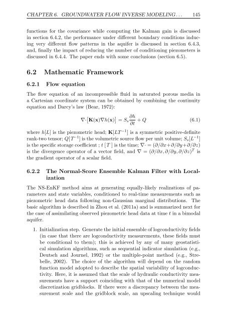
The flow equation of an incompressible fluid in saturated porous media in
a Cartesian coordinate system can be obtained by combining the continuity
equation and Darcy’s law (Bear, 1972):
∇· [ K(x)∇h(x) ] ∂h
= Ss + Q (6.1)
∂t
where h[L] is the piezometric head; K[LT −1 ] is a symmetric positive-definite
rank-two tensor; Q[T −1 ] is the volumetric source flow per unit volume; Ss[L −1 ]
is the specific storage coefficient ; t [T ] is the time; ∇· = (∂/∂x+∂/∂y+∂/∂z)
is the divergence operator of a vector field, and ∇ = (∂/∂x, ∂/∂y, ∂/∂z) T is
the gradient operator of a scalar field.
6.2.2 The Normal-Score Ensemble Kalman Filter with Localization
The NS-EnKF method aims at generating equally-likely realizations of parameters
and state variables, conditioned to real-time measurements such as
piezometric head data following non-Gaussian marginal distributions. The
basic algorithm is described in Zhou et al. (2011a) and is summarized next for
the case of assimilating observed piezometric head data at time t in a bimodal
aquifer.
1. Initialization step. Generate the initial ensemble of logconductivity fields
(in case that there are logconductivity measurements, these fields must
be conditional to them); this is achieved by any of many geostatistical
simulation algorithms, such as sequential indicator simulation (e.g.,
Deutsch and Journel, 1992) or the multiple-point method (e.g., Strebelle,
2002). The choice of the algorithm will depend on the random
function model adopted to describe the spatial variability of logconductivity.
Here, it is assumed that the scale of hydraulic conductivity measurements
have a support coinciding with that of the numerical model
discretization gridblocks. If there were a discrepancy between the measurement
scale and the gridblock scale, an upscaling technique would