Upscaling and Inverse Modeling of Groundwater Flow and Mass ...

14 CHAPTER 2. A COMPARATIVE STUDY OF THREE- . . .
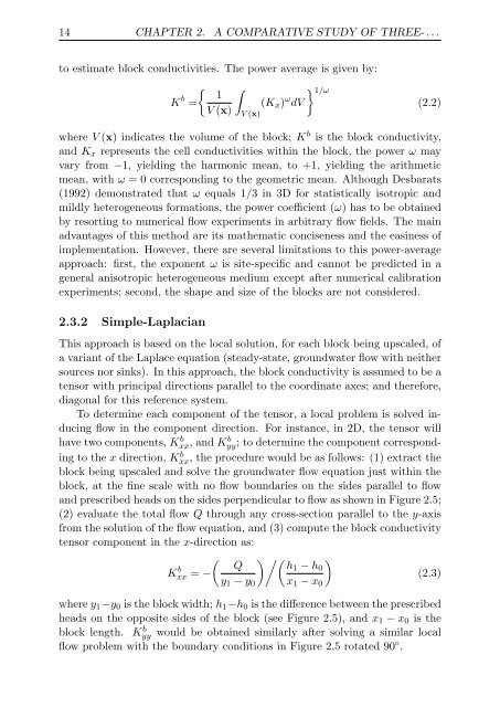
to estimate block conductivities. The power average is given by:
K b { ∫
1
=
(Kx)
V (x) V (x)
ω } 1/ω
dV
(2.2)
where V (x) indicates the volume of the block; K b is the block conductivity,
and Kx represents the cell conductivities within the block, the power ω may
vary from −1, yielding the harmonic mean, to +1, yielding the arithmetic
mean, with ω = 0 corresponding to the geometric mean. Although Desbarats
(1992) demonstrated that ω equals 1/3 in 3D for statistically isotropic and
mildly heterogeneous formations, the power coefficient (ω) has to be obtained
by resorting to numerical flow experiments in arbitrary flow fields. The main
advantages of this method are its mathematic conciseness and the easiness of
implementation. However, there are several limitations to this power-average
approach: first, the exponent ω is site-specific and cannot be predicted in a
general anisotropic heterogeneous medium except after numerical calibration
experiments; second, the shape and size of the blocks are not considered.
2.3.2 Simple-Laplacian
This approach is based on the local solution, for each block being upscaled, of
a variant of the Laplace equation (steady-state, groundwater flow with neither
sources nor sinks). In this approach, the block conductivity is assumed to be a
tensor with principal directions parallel to the coordinate axes; and therefore,
diagonal for this reference system.
To determine each component of the tensor, a local problem is solved inducing
flow in the component direction. For instance, in 2D, the tensor will
have two components, K b xx, and K b yy; to determine the component corresponding
to the x direction, K b xx, the procedure would be as follows: (1) extract the
block being upscaled and solve the groundwater flow equation just within the
block, at the fine scale with no flow boundaries on the sides parallel to flow
and prescribed heads on the sides perpendicular to flow as shown in Figure 2.5;
(2) evaluate the total flow Q through any cross-section parallel to the y-axis
from the solution of the flow equation, and (3) compute the block conductivity
tensor component in the x-direction as:
(
Q
)/( )
h1 − h0
K b xx = −
y1 − y0
x1 − x0
(2.3)
where y1−y0 is the block width; h1−h0 is the difference between the prescribed
heads on the opposite sides of the block (see Figure 2.5), and x1 − x0 is the
block length. K b yy would be obtained similarly after solving a similar local
flow problem with the boundary conditions in Figure 2.5 rotated 90 ◦ .